48. Liu, Z., and P. Bird, Finite element modeling of neotectonics in New Zealand, J. Geophys. Res., 107(B12), 2328, doi:10.1029/2001JB001075, 2002(a).

Abstract. Thin-shell finite element methods that incorporate faults, realistic rheology, laterally varying heat flow and topography, and plate velocity boundary conditions have been used to model the neotectonics of New Zealand. We find that New Zealand’s faults have effective friction of 0.17, comparable to that found in other Pacific Rim regions. The long-term average slip rate of the Alpine fault varies along strike, generally increasing northeastward until slip is partitioned among the strands of the Marlborough system. The average slip rate, 30 mm/yr, when combined with published geodetic results and historical seismicity, strongly suggests a high probability of future large earthquakes. Tectonic deformation of North Island is controlled by a balance between differential topographic pressure and traction from the Hikurangi subduction thrust. The Hikurangi forearc is an independent plate sliver moving relative to the Pacific and Australian plates. There is a complicated zone of slip partitioning in the transition from the Alpine fault to the Puysegur trench. An offshore thrust fault, the southern segment of which may correspond to the Waipounamou fault system, parallels to the SE coast of South Island and needs to be included in seismic hazard estimates.

Acknowledgement: This material is based upon work supported by the National Science Foundation under Grant No. 9902735. Any opinions, findings and conclusions or recomendations expressed in this material are those of the author(s) and do not necessarily reflect the views of the National Science Foundation (NSF).

Entire paper as a 887 KB .pdf file (18 pages, black-and-white)

Following are a complete set of figures for this paper, in bitmap form. Note that many are larger, and more legible, than the versions provided by JGR in the on-line HTML version.

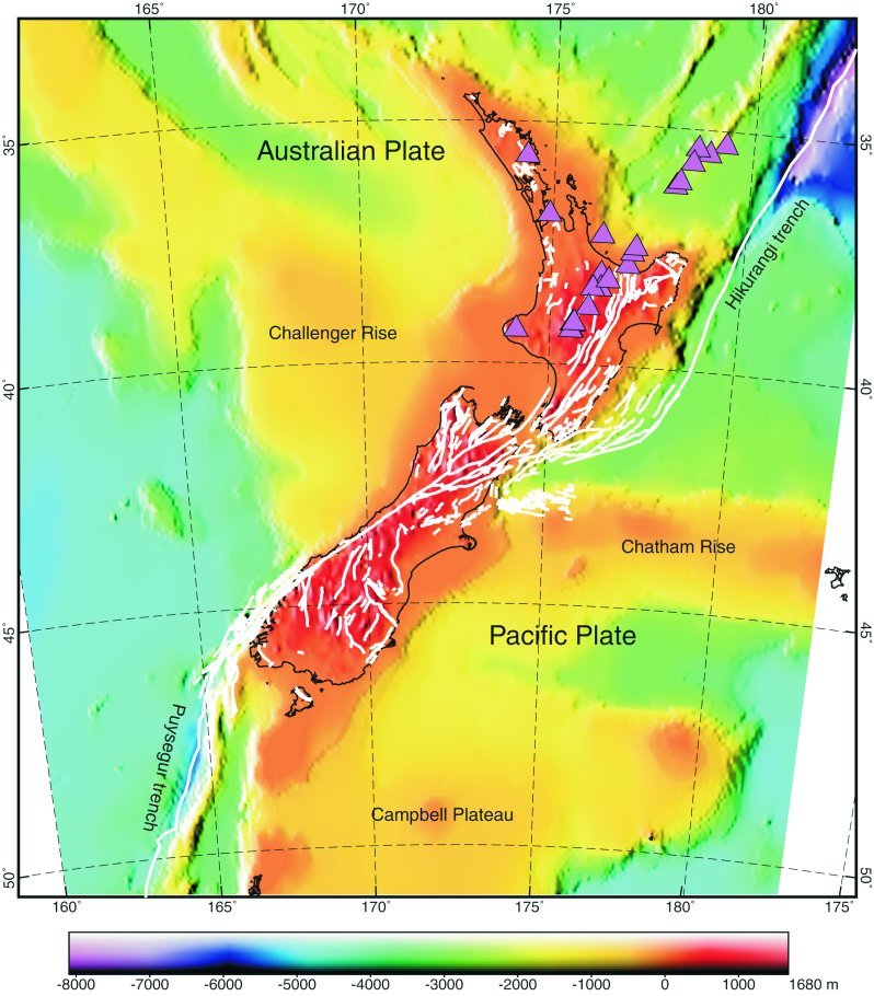
Figure 1. Tectonic environment of New Zealand. Lambert conformal conic projection. Major tectonic elements are labeled. White lines represent active and potentially active fault traces. Triangles represent active volcanoes overlying shaded-relief topography. The hypothesized northwestern and southeastern faults offshore South Island are not shown in this figure; compare to Figure 3.

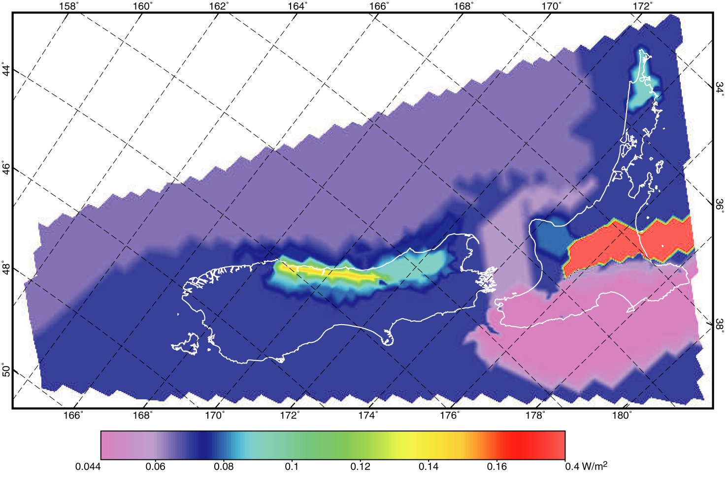
Figure 2. Contours of nonuniform heat flow map used in the final model group 7. Mercator projection. Values range from 0.044 to 0.4 W/m². Exceptionally high heat flow is concentrated in the Taupo Volcanic Zone and assumed to be 0.4 W/m². High heat flow in the Southern Alps is caused primarily by extremely high erosion rates.

Figure 3. A typical finite element grid used in neotectonic modeling of New Zealand. Mercator projection. Thin lines and thick lines represent continuum elements and fault elements, respectively. Symbols on the fault traces represent fault type: open triangle, thrust fault; solid triangle, subduction thrust fault; solid square, fault with dip angle 45º; short tick, normal fault. Faults without symbols attached are strike-slip faults. Fault dips are assigned: 90º (strike-slip fault), 65º (normal fault), 30º (thrust fault), and 25º (subduction thrust fault). Subduction thrust fault is subject to a limit (Taumax) on the downdip integral of shear traction. All faults including hypothesized NW and SE coastal faults offshore South Island are shown.

Figure 4. Model scores versus fault friction. Both uniform heat flow (70 mW/m²) and nonuniform heat flow maps are used. The total misfit error is obtained according to the score formula in the text. The optimal model should give low mean stress azimuth, GPS, and slip rate misfit error. (a) Mean stress azimuth misfit error versus fault friction. Diamond represents uniform heat flow case. Triangle represents nonuniform heat flow case. Same symbol notation is used in (b) –(d). (b) GPS misfit error versus fault friction. (c) Fault slip rate misfit error versus fault friction. (d) Total misfit error versus fault friction. The gray bar indicates compromise values for fault friction.

Figure 5. Model scores versus dip angle of central Alpine fault. Both uniform heat flow (70 mW/m²) and nonuniform heat flow maps are used. The total misfit error is obtained according to the score formula in the text. (a) Mean stress azimuth misfit error versus dip angle of central Alpine fault. (b) GPS misfit error versus dip angle of central Alpine fault. (c) Fault slip rate misfit error versus dip angle of central Alpine fault. (d) Total misfit error versus dip angle of central Alpine fault. Same symbol notation is used as in Figure 4 for (a) –(d), in which diamond and triangle represent uniform heat flow and nonuniform heat flow cases, respectively.

Figure 6. Prediction errors with a fixed northeastern boundary (fixed b.c.) on the Hikurangi forearc versus prediction errors with a ‘‘free’’ boundary condition (‘‘free’’ b.c.) at the same part of boundary within various model groups. Each triangle corresponds to a pair of models (‘‘free’’ b.c. and fixed b.c. cases) with the other model parameters being the same. The legend besides each point gives labels of each model pair. The dashed line shows the line on which the different boundary conditions are not differentiable. Generally, models with ‘‘free’’ b.c. on the northeastern boundary of Hikurangi forearc have lower errors and thus are more realistic than models with fixed b.c.

Figure 7. (a) Surface velocity predicted by the preferred model NZT001. (b) Surface velocity of comparison model NZT003. Mercator projection. Both of them use the same parameters: fault friction 0.17, dip angle in the central Alpine fault 50º, traction "free" boundary condition on the NE boundary of Hikurangi forearc. But the downdip integral of interplate shear traction/unit-strike for model NZT001 (7.5x10¹² N/m) is 3 times greater than that assumed in comparison model NZT003. Fast extension resulting from topographic pressure has to be balanced by shear tractions imposed by oblique subduction. To increase legibility, different scaling is used when plotting velocity vectors in (a) and (b).

Figure 8. Continuum strain rates (expressed as microfault orientations) from the preferred thin-shell model NZT001. Mercator projection. Dumbbell symbols shows conjugate thrust faulting; X symbols shows conjugate strike-slip faulting; blank rectangles shows conjugate normal faulting. The fault symbols are plotted with area proportional to strain rate. Thinning factor 1/7 is used to reduce the number of symbols and increase legibility.

Figure 9. Most compressive horizontal principal stress directions predicted by the best thin-shell model NZT001. Mercator projection. Open rectangle bars represent normal faults, gray bars represent strike-slip faults, and dark filled bars represents thrust faults. Thinning factor 1/14 is used to reduce the number of symbols and increase legibility.

Figure 10. Long-term average fault slip rates predicted by preferred model NZT001. Mercator projection. The width of each ribbon plotted beside a fault is proportional to long-term slip rate, which is also given by numbers in mm/yr. Faults with very small slip rates are locked and not marked by slip rates in the figure. The different colors of ribbon represents normal, thrust, dextral, and sinistral faulting, respectively.