46. Bird, P., Y. Y Kagan, and D. D. Jackson, (2002) Plate tectonics and earthquake potential of spreading ridges and oceanic transform faults, in: S. Stein and J. T. Freymueller (editors), Plate Boundary Zones, Geodynamics Series , 30, 203-218, Am. Geophys. U., Washington, DC.
Abstract. We use the Harvard CMT catalog to separate ocean-ridge seismicity into spreading and transform sub-catalogs. We use the tapered Gutenberg-Richter distribution to estimate the total seismic moment rates of plate-boundary zones from limited catalogs of large events. We present the plate boundary model PB1999 and use it to associate marine earthquakes with particular plate boundary segments. We then combine these tools to estimate corner magnitudes (mc), spectral slopes (b ), and coupled lithosphere thicknesses for all spreading ridges and oceanic transform faults. The distribution of spreading earthquakes is consistent with "normal" b (although b is not well constrained) and with uniform mc = 5.8. Coupled lithosphere thickness along ridges decreases quasi-exponentially (from about 500 m to under 50 m) as spreading rate increases. Oceanic transform faults also have "normal" b , but their corner magnitudes decrease from about 7.1 to about 6.3 with increasing relative plate velocity. Oceanic transform faults also show a quasi-exponential decrease in coupled lithosphere thickness (from about 3000 m to about 300 m) as relative plate velocity increases. Perhaps this is due to formation of serpentine along slow ridges and transforms and its absence from fast ridges and transforms. Spreading ridges and oceanic transform faults both have imperfect seismic coupling because: (i) all detailed local studies of seismogenic lithosphere thickness exceed our mean values for coupled thickness, and (ii) if coupling were perfect, and seismogenic lithosphere thickness were as small as our estimated coupled thickness, it would require unreasonable stress drops or rupture shapes to explain the moments of the largest earthquakes.
P.S.
We speculated in this paper that alteration of exposed mantle to serpentine at slow-spreading ridges (like the Gakkel Ridge) may explain their higher seismic coupling. We also noted that the Romanche transform fault system has the highest coupling (~1) of all oceanic transforms. Soon after this went to press, Bonatti et al. (2001, Geology, 29, #11) showed that oceanic crust is thin or absent along the Romanche transform and fracture zone. P. Bird, 2001.12.03Entire paper as a 2 MB .pdf file

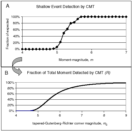
Figure 1. Estimated detection rates for shallow events in the Harvard CMT catalog. Part A (top), estimated fraction of events ![]() detected at each magnitude. This was computed by fitting a tapered Gutenberg-Richter distribution to all shallow events in the complete part of the catalog, and then assuming that the same parameters
detected at each magnitude. This was computed by fitting a tapered Gutenberg-Richter distribution to all shallow events in the complete part of the catalog, and then assuming that the same parameters ![]() and
and ![]() would describe the statistics of smaller events if detection were perfect. Part B (bottom), moment recording factors R (fraction of actual scalar seismic moment expected to appear in the catalog) for various corner magnitudes
would describe the statistics of smaller events if detection were perfect. Part B (bottom), moment recording factors R (fraction of actual scalar seismic moment expected to appear in the catalog) for various corner magnitudes ![]() , based on the upper part of the figure.
, based on the upper part of the figure.
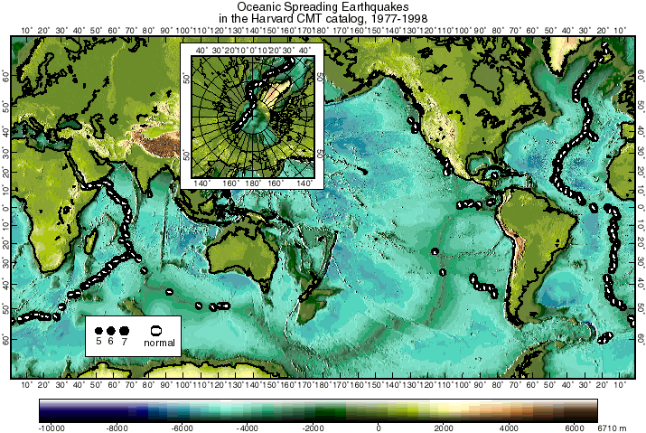
Figure 2. Global distribution of spreading earthquakes (beachballs), as defined in the text, during 1977-1998 inclusive, in the Harvard CMT catalog. Inset shows Arctic region. Beachballs show lower focal hemisphere projections of the double-couple part of the moment tensor. Note that the fast-spreading East Pacific Rise has very few spreading earthquakes, while the slow-spreading Mid-Atlantic Ridge has many.
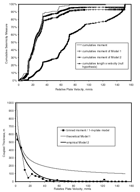
Figure 3. Cumulative (top) and differential (bottom) distributions of spreading earthquake moment as a function of relative plate velocity, and various models to explain them. The cumulative distribution is normalized to the total of 1.31´ 1020 N m for the 22-year period. Differential (frequency histogram) distribution was created by binning earthquake moments into 5 mm/a-wide spreading-velocity bins, and then dividing these moment sums by the theoretical moment produced by a 1-m-thick lithosphere to get apparent coupled thickness. The null hypothesis is that all ridges have equal coupled thickness and produce moment in proportion to length ´ velocity, but this is clearly incorrect. Model 1 (self-similar) has coupled lithosphere thickness decreasing as inverse square root of velocity, and corner magnitude decreasing as log of velocity. Model 2 has constant corner magnitude, but an exponential decrease in coupled thickness with increasing velocity. Both models are corrected for imperfect moment detection, using the ![]() function from Figure 1B.
function from Figure 1B.
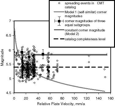
Figure 4. Spreading earthquake magnitudes versus relative plate velocity. The Model 1 curve has the predicted form ![]() , which can be rejected. Squares show maximum-likelihood corner magnitudes for three sub-catalogs of roughly equal size. All evidence seems consistent with a uniform corner magnitude of 5.82 for spreading earthquakes.
, which can be rejected. Squares show maximum-likelihood corner magnitudes for three sub-catalogs of roughly equal size. All evidence seems consistent with a uniform corner magnitude of 5.82 for spreading earthquakes.
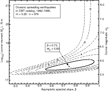
Figure 5. Maximum-likelihood determination of the tapered Gutenberg-Richter parameters ![]() and
and ![]() for spreading earthquakes in 1982-1998 inclusive with
for spreading earthquakes in 1982-1998 inclusive with ![]() . The method is described by equation (12) of Kagan and Jackson [2000]. Contours show parameter combinations of equal likelihood; the contour labeled "0" corresponds to
. The method is described by equation (12) of Kagan and Jackson [2000]. Contours show parameter combinations of equal likelihood; the contour labeled "0" corresponds to ![]() and thus defines the 95%-confidence region. Uncertainties stated in this paper are the horizontal and vertical dimensions of the region bounded by this contour.
and thus defines the 95%-confidence region. Uncertainties stated in this paper are the horizontal and vertical dimensions of the region bounded by this contour.
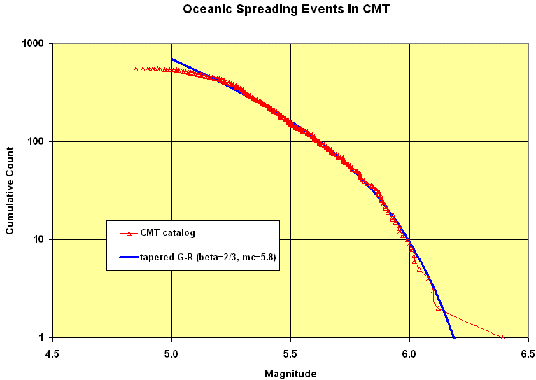
Figure 6. Fit of a tapered Gutenberg-Richter distribution (equation 3, with ![]() and
and ![]() ) to the frequency-magnitude relation for spreading earthquakes in the Harvard CMT catalog, 1977-98. Since the corner magnitude is so close to the catalog threshold, no part of the distribution is free of the effects of the corner-magnitude term, and
) to the frequency-magnitude relation for spreading earthquakes in the Harvard CMT catalog, 1977-98. Since the corner magnitude is so close to the catalog threshold, no part of the distribution is free of the effects of the corner-magnitude term, and ![]() cannot be determined with high confidence. (However, it is less than the slope obtained by fitting a straight-line Gutenberg-Richter distribution.)
cannot be determined with high confidence. (However, it is less than the slope obtained by fitting a straight-line Gutenberg-Richter distribution.)
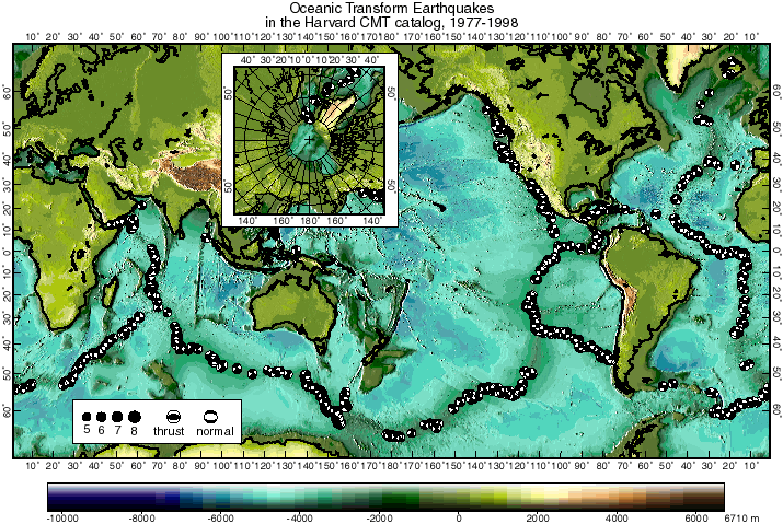
Figure 7. Global distribution of oceanic transform earthquakes (beachballs), as defined in the text, during 1977-1998 inclusive, in the Harvard CMT catalog. Inset shows Arctic region. Beachballs show lower focal hemisphere projections of the double-couple part of the moment tensor.
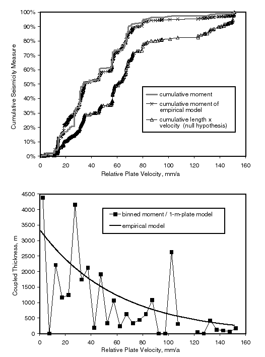
Figure 8. Cumulative (top) and differential (bottom) distributions of oceanic transform earthquake moment as a function of relative plate velocity, and two models to explain them. Cumulative curves are normalized to the total of 2.20´ 1021 N m for the 22-year period. Differential (frequency histogram) distribution was created by binning earthquake moments into 5 mm/a-wide transform-velocity bins, and then dividing these moment sums by the theoretical moment produced by a 1-m-thick lithosphere to get apparent coupled thickness. The null hypothesis is that all transforms have equal coupled thickness and produce moment in proportion to length ´ velocity, but this is clearly incorrect. Our empirical model has corner magnitude declining slightly with increasing velocity, and an exponential decrease in coupled thickness with increasing velocity. Both models are corrected for imperfect moment detection, using the ![]() function from Figure 1B.
function from Figure 1B.
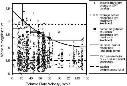
Figure 9. Magnitudes of oceanic transform earthquakes versus relative plate velocity. The catalog is only complete for ![]() , and the corner magnitude for the whole group is 6.9. Corner magnitudes for three equal-sized subgroups (squares) show an important reduction of corner magnitude with velocity. An empirical quadratic form has been fit to these values.
, and the corner magnitude for the whole group is 6.9. Corner magnitudes for three equal-sized subgroups (squares) show an important reduction of corner magnitude with velocity. An empirical quadratic form has been fit to these values.
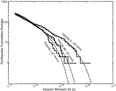
Figure 10. Fits of tapered Gutenberg-Richter frequency-moment distributions (equation (3); dotted curves) to the oceanic transform earthquake catalog, after division into three subgroups on the basis of relative plate velocity. Spectral slope b is in the range 0.60-0.65 for each curve, but corner magnitude ![]() decreases from 7.06 to 6.59 to 6.37 as velocity increases.
decreases from 7.06 to 6.59 to 6.37 as velocity increases.