52. Liu, Z., and P. Bird, Two-dimensional and three-dimensional finite element modelling of mantle processes beneath central South Island, New Zealand, Geophys. J. Int., 165, 1003-1028, 2006.

Abstract. Numerical models that include pre-existing faults, elasto–visco–plastic rheology, thermal structure, realistic plate boundary conditions, and surface erosion are built to investigate alternative hypotheses of mantle flow geometry beneath central South Island, New Zealand. Bouguer gravity anomalies, teleseismic traveltime delays and seismic velocity structures are used to constrain models. Model predictions are compared with topography, uplift, magnetotelluric resistivity structure, isostatic gravity anomalies (IGAs), and seismicity.We find that the wedge model, in which the mantle lithosphere of the Australia plate is wedged between crust and mantle lithosphere of the Pacific plate, gives reasonable predictions of topography, uplift rate, IGAs, and stress and strain state in the lithosphere. Coupled erosional-tectonic models suggest that tectonic compression primarily determines the asymmetric surface relief, with erosion influencing its detail and having small effects on shallow stresses. Both 2-D and 3-D models suggest that the neotectonics of central South Island is dominated by weak faults. 3-D model results show that the Alpine fault and mantle shear zone accommodate most convergent and strike-slip plate motion, confirming non-partitioned plate motion in this region. Adding the regional strike-slip component has little effect on the convergent velocity field, and only changes the stress field by rotating the horizontal principal stresses out of the plane of the cross-section.

Acknowledgement: This material is based upon work supported by the National Science Foundation under Grant No. 9902735. Any opinions, findings and conclusions or recomendations expressed in this material are those of the author(s) and do not necessarily reflect the views of the National Science Foundation (NSF).

N.B. Blackwell Publishing (GJI) does not permit posting the .pdf file online.  If you cannot get the paper through regular channels, I encourage you to e-mail Zhen Liu or myself.

Following are a complete set of figures for this paper, in bitmap form.

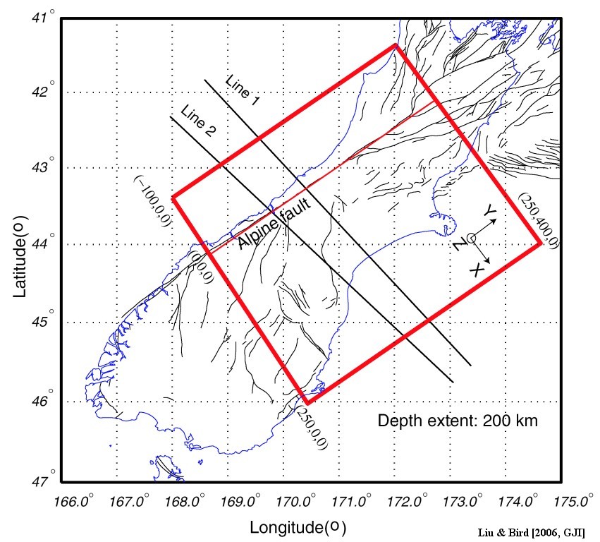
Figure 1. Model domain in 2-D plane view. The rectangular box shows model domain: 400 km in length (along the strike of Alpine fault), 350 km in width (across the Island), and 200 km in depth. Local Cartesian coordinate system is shown with +x-axis across the island, +y-axis along the strike, and +z axis pointing up. The origin of coordinates (0, 0, 0) is chosen to be southwestern endpoint of the Alpine fault. Line 1, 2 are two geophysical profiles of the SIGHT (New Zealand South Island Geophysical Transect) experiment. Thin lines represent faults.

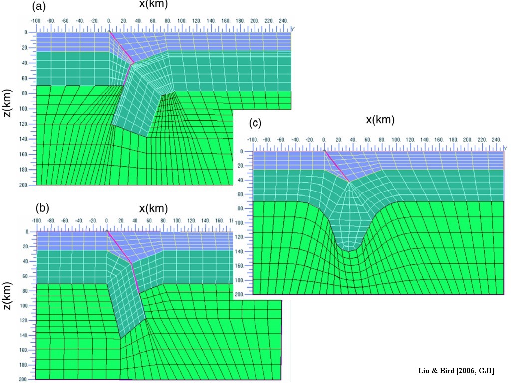
Figure 2. X–z cross-sections of subsurface geometries and finite element meshes of three mantle models. 2 km fault zone located at x = [0, 2] km is meshed with 1-km-wide elements. The model domain has a width of 250 km and a depth of 200 km. (a) wedge model, in which Australia plate acts as an indention block to force Pacific crust to delaminate from Pacific mantle; (b) Australia plate subduction model (“subduction model”). Australia plate subducts beneath Pacific plate; (c) Homogeneous shortening and distributed shearing model (“shearing model”). These three models share a similar crust structure constrained by seismic studies (Scherwath et al. 2002).

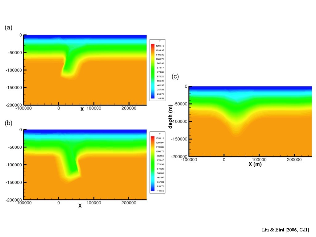
Figure 3. Thermal structures of the three mantle models. (a)Wedge model; (b) Subduction model; (c) Shearing model. Thermal structures of (a), (b) are derived by advecting steady state pro-orogenic geotherms along the convergent plates. The steady state geotherm is obtained by assuming the surface heat flow 70 mW m⁻² and the bottom of the lithosphere being on the isotherm 1250^◦C. The heat conductivities and heat productions are global average values from thin-shell modelling. Thermal perturbation caused by uplift and erosion and shear heating near Alpine fault are neglected. Hypothetical thermal structures due to shortening and thickening are used in (c).  3-D thermal structures are derived by extrapolating 2-D thermal structure on x–z cross-section along +y direction.

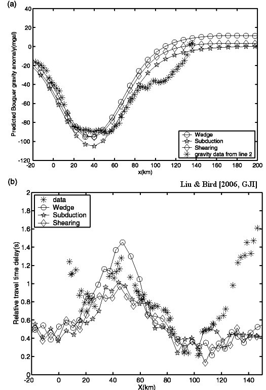
Figure 4. (a) Predicted Bouguer gravity anomalies on the surface from three mantle models versus observation from line 2. The reference density column is assumed as 0–25 km (crust: 2816 kg m⁻³), 25–70 km (mantle lithosphere: 3332 kg m⁻³), 70–200 km (asthenosphere: 3270 kg m⁻³). (b) Computed and observed relative P-wave traveltime delays along Line 1 in SIGHT from Honshu earthquakes. The observed delays are from Stern et al. (2000). The deviation to the west of +20 km and east of +100 km is due to the absence of shallow sediment structures in our models.

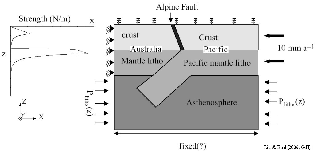
Figure 5. Boundary conditions in x–z cross-section. The strength profile with depth is shown alongside. For the wedge and shearing models, constant plate velocity is imposed on the side of Pacific lithosphere and the Australia plate side remains fixed. For the subduction model, the Australia plate moves and the Pacific plate is fixed. Winkler restoring force is used at the surface (maximum density contrast interface) to simulate isostatic adjusting forces.  Different boundary conditions are imposed at the bottom of the model domain: fixed, roller, and constant flux. In the 3-D model, along +y (pointing into the paper), strike-parallel and convergent components from NUVEL1-A are imposed. Lithostatic pressure boundary conditions are also imposed on at y = 0 and y = +400 km plane in asthenosphere in 3-D models. The other boundaries of the asthenosphere share the same pressure boundary condition as in the 2-D model.

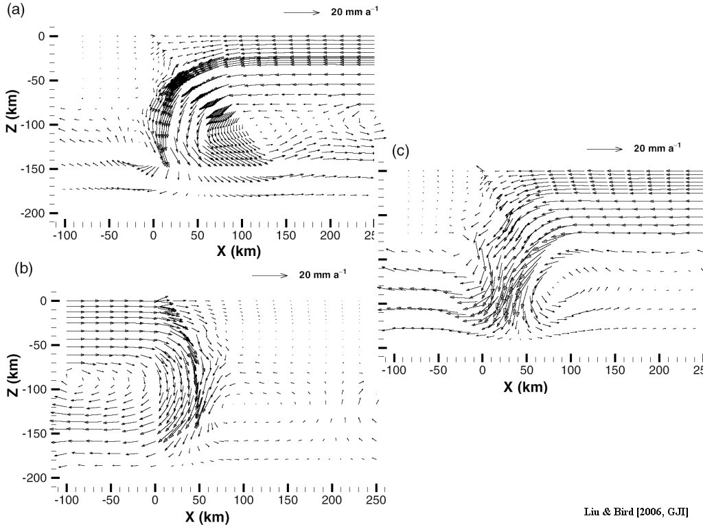
Figure 6. Velocity fields of three mantle processes in the reference model set M0. (a) Wedge; (b) subduction and (c) shearing.

Figure 7. Predicted topography of three mantle models versus averaged topography in the reference model. Both correlation and misfit errors are listed. The wedge model gives a good fit of topography shape and overall minimum misfit error.

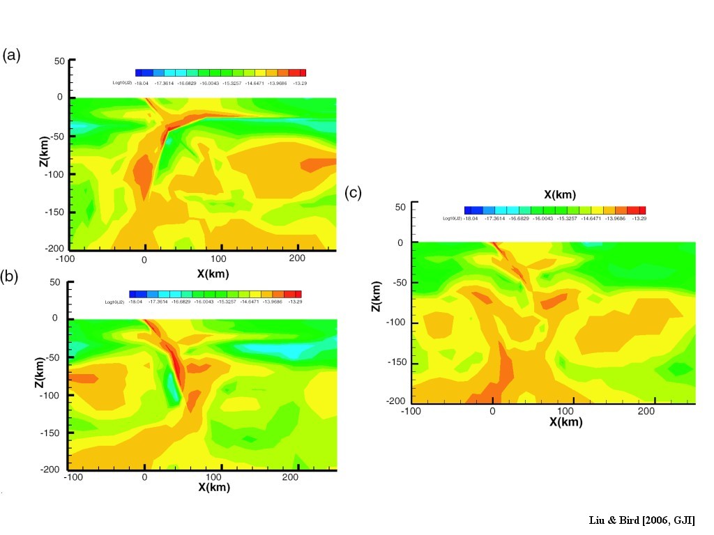
Figure 8. Predicted logarithm of the second invariant of strain rate tensor in the reference models. (a), (b), (c) correspond to wedge, subduction, and shearing model, respectively. The doubly vergent shearing band is clearly seen in the wedge model, which agrees well with magnetotelluric models.

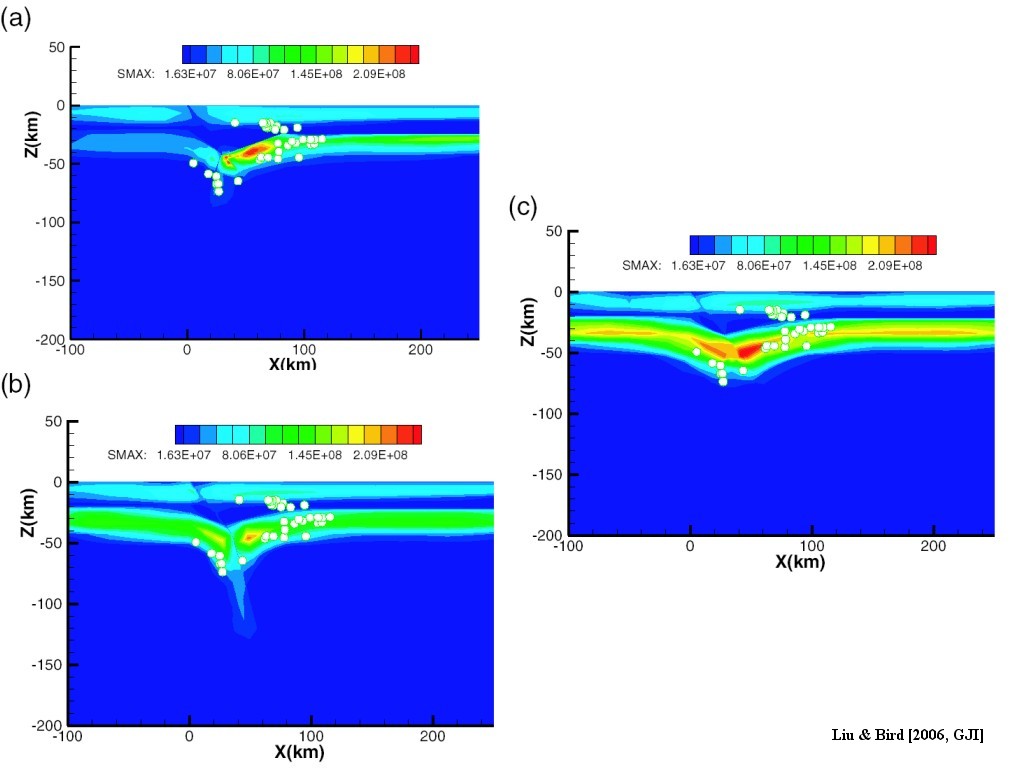
Figure 9. Maximum shear stress in three mantle models. The white circles represent 2-D projection of earthquakes recorded by Pukaki network (Reyners 1987). In general, there is good coincidence between earthquake locations and high shear stress zones, except in the southeast-dipping earthquake cluster at depths of 14–25 km, which may be caused by some local effects.

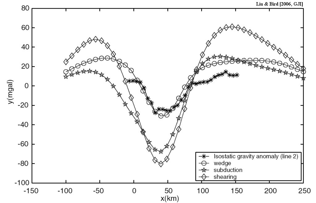
Figure 10. Predicted IGAs for three models versus IGA data along line 2. The data is from the gravity map of New Zealand 1:1,000,000 (Department of Scientific and Industrial Research, Wellington, New Zealand, 1977). The isostatic correction is based on the Airy-Heiskanen system with assumed crustal thickness at sea level 25 km, and elevation effect is included. The wedge model predicts minimum IGA ~ −30 mgal, and ~ +10 mgal adjacent to Alpine fault (x = 0 km), consistent with observation (Stern 1995).

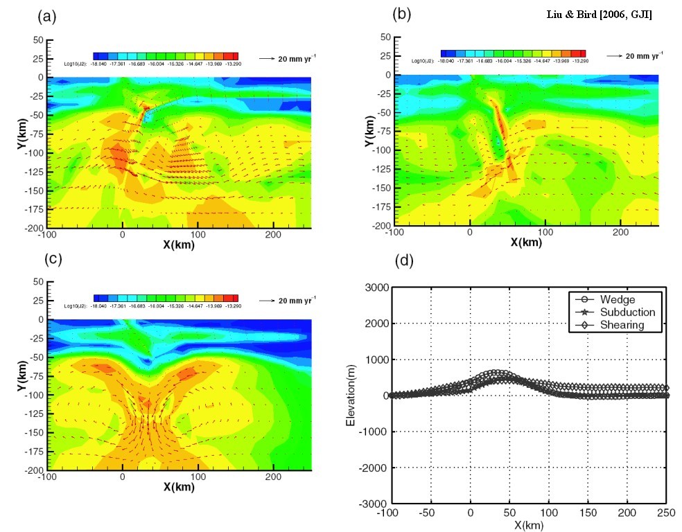
Figure 11.  Predicted logarithm of the second invariant of strain rate tensor by the models with no convergence imposed. The strain rate field is overlaid with velocity field shown as red vectors. (a) wedge model; (b) subduction model; (c) shearing model. Predicted topography at the end of 1 Myr from three models is shown in (d).

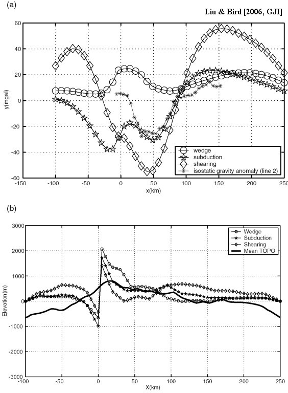
Figure 12.  (a) Predicted isostatic gravity anomaly of model M1, in which a dry diabase crust is assumed. (b) Predicted topography of model M24, in which wet Anhem dunite is assumed for the mantle lithosphere rheology.

Figure 13.  Predicted topography, isostatic gravity anomaly, strain rate, and maximum shear stress of the shearing model with “softer” mantle lithosphere. The viscosity of the mantle lithosphere is reduced by a factor of 10 through a reduction of the A parameter in the dislocation creep law. Boundary conditions and crust rheology are the same as in reference model M0. (a) Predicted topography versus averaged topography; (b) Predicted isostatic gravity anomaly versus data along SIGHT line 2; (c) logarithm of the second invariant of strain rate tensor overlaid with velocity vectors (red vector); (d) maximum shear stress in the shearing model. The reduction of viscosity in the mantle lithosphere reduces the stress level to ~80 Mpa.

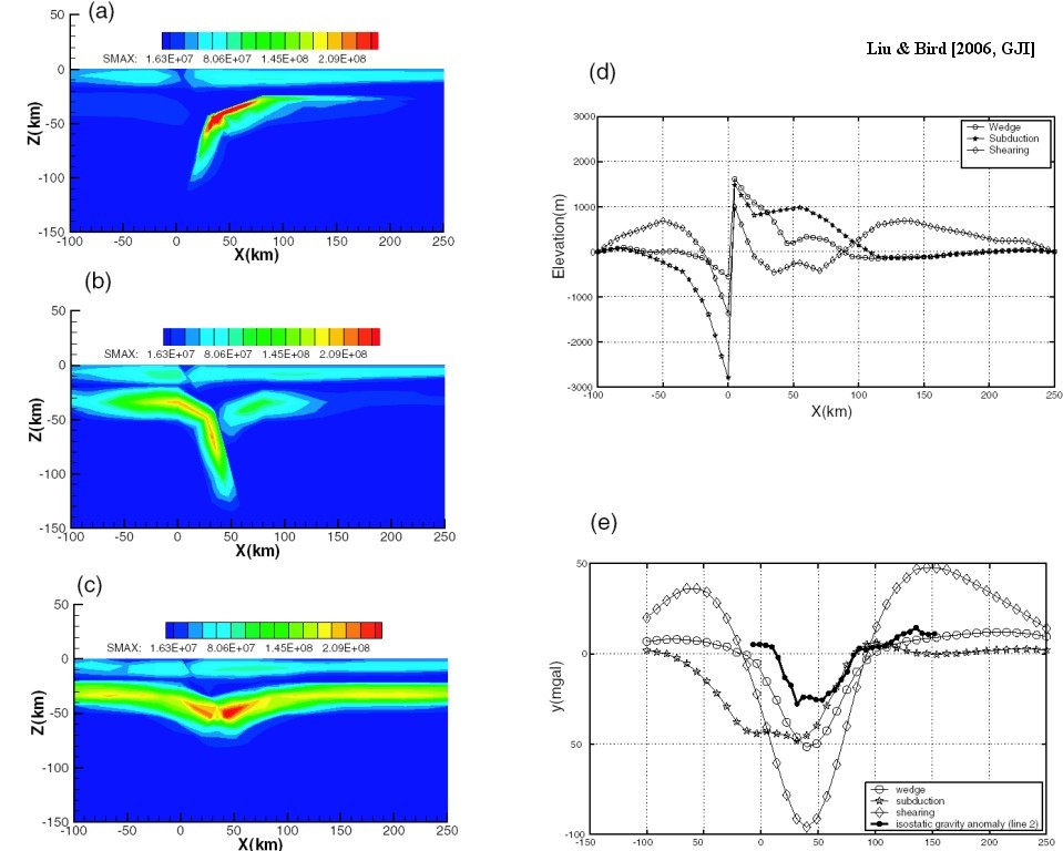
Figure 14. Predicted maximum shear stress, topography, and isostatic gravity anomaly of model M22, in which a lower asthenosphere viscosity 2 × 10¹⁹Pa s is assumed. (a), (b) and (c) gives maximum shear stress level in the wedge model, subduction and shearing model, respectively. (d) Predicted topography from these three models; (e) Predicted isostatic gravity anomalies from these three models.

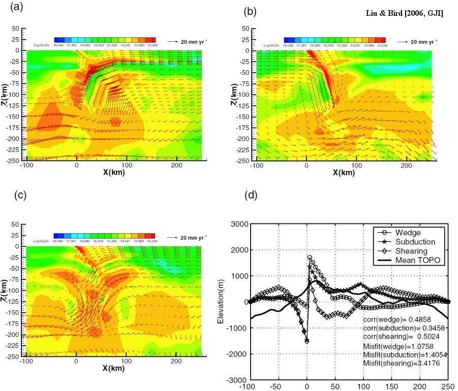
Figure 15.  Predicted logarithm of the second invariant of strain rate tensor (a)–(c) and surface topography (d) in model M27. The fixed bottom boundary has been extended to z = −600 km instead of z = −200 km in the reference model. (a) wedge model; (b) subduction model and (c) shearing model; (d) predicted topography from three models. The velocity is overlaid on the strain rate plot in (a), (b) and (c). Only the top 250 km of the model domain is shown.

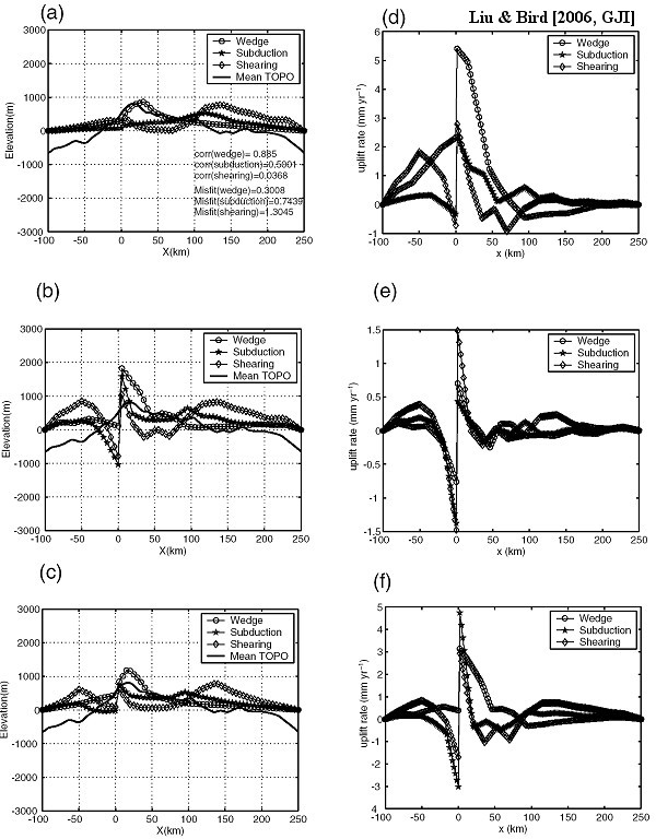
Figure 16.  Predicted topography and surface uplift rate in one coupled tectonic-erosion model, in which effective diffusivity of 3 m² yr⁻¹, transport coefficient of 3, and extract efficiency of 1 × 10⁸ m² are used. (a), (d) give predicted topography, surface uplift rate under joint effects of diffusion, and fluvial transport.  (b), (e) give topography, uplift rate with diffusion only; (c), (f) give topography, uplift rate predictions with fluvial transport only. The wedge model predicts the highest uplift rate adjacent to the Alpine fault (x = 0) with decreasing rate to <1 mm yr^-1 50 km away as shown in (a) (d).

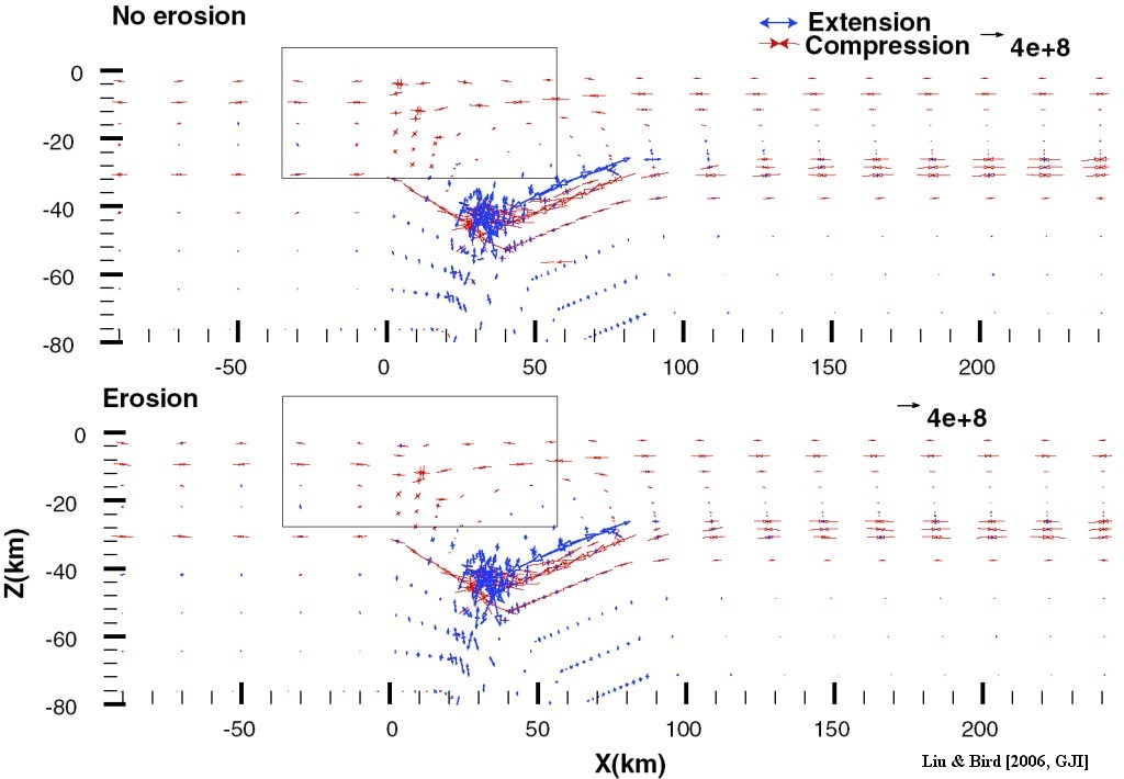
Figure 17.  Stress anomalies from the coupled tectonic-erosion wedge model vs. pure tectonic wedge model, in Pa. The stress anomaly tensor is calculated by subtracting a reference depth-dependent lithostatic pressure from the final stress tensor solution. Principal stress directions are plotted. Convergent and divergent arrow pairs represent compression and extension, respectively. The arrow length is proportional to the size. The rectangle indicates the region where differences in stress anomaly occur. The loading/unloading due to surface erosion-induced mass change does not have significant influence on stress states in the lithosphere.

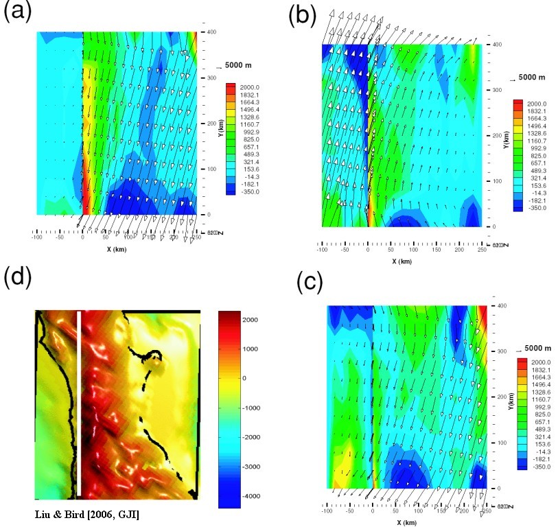
Figure 18.  Predicted topography in 3-D models versus surface topography in model domain. The x–y plane (surface) view is shown. Arrows represent the projected surface displacement vectors. Colour contours represent the accumulated vertical displacement. (a) Wedge; (b) Subduction; (c) Shearing model; (d) Surface topography from ETOPO5.

Figure 19.  Predicted isostatic gravity anomalies at the surface from 3-D models versus isostatic gravity anomaly data in the model domain. (a) Wedge; (b) Subduction; (c) Shearing model; (d) Observed isostatic gravity anomalies in model domain (regular box in Fig. 1) from Gravity Map of New Zealand 1:1,000,000 (Department of Scientific and Industrial Research, Wellington, New Zealand, 1977). Mercator Projection. Thin white line in (d) represents Alpine fault trace.  Corresponding location of Alpine fault in local Cartesian system (a) and Mercator projection plot (d) is indicated. The wedge model gives a good prediction of decreasing isostatic gravity anomaly from northeast to southwest, and anomaly magnitude.

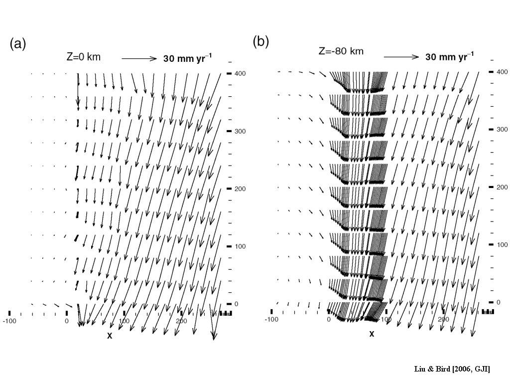
Figure 20.  Cross-sections at depth of 3-D velocity field from the wedge model. (a) At the surface (z = 0 km); (b) At z = −80 km. Note that large vectors near y = 0 or 400 km in the Alpine fault are due to boundary effects.

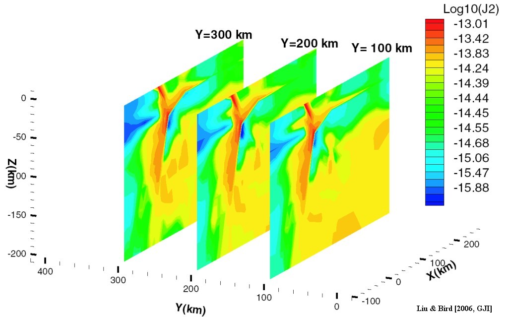
Figure 21.  The logarithm of the second invariant of strain rate tensor of the 3-D wedge model at the cross-sections at y = 100, 200 and 300 km.