75. Bird, P. [2017] Stress field models from Maxwell stress functions: southern California, Geophys. J. Int., 210(2), 951-963, doi: 10.1093/gji/ggx207.
Abstract. The lithospheric stress field is formally divided into three components: a standard pressure which is a function of elevation (only), a topographic stress anomaly (3-D tensor field), and a tectonic stress anomaly (3-D tensor field). The boundary between topographic and tectonic stress anomalies is somewhat arbitrary, and here is based on the modeling tools available. The topographic stress anomaly is computed by numerical convolution of density anomalies with three tensor Green’s functions provided by Boussinesq, Cerruti, and Mindlin. By assuming either a seismically-estimated or isostatic Moho depth, and by using Poisson ratio of either 0.25 or 0.5, I obtain 4 alternative topographic stress models. The tectonic stress field, which satisfies the homogeneous quasi-static momentum equation, is obtained from particular second-derivatives of Maxwell vector potential fields which are weighted sums of basis functions representing constant tectonic stress components, linearly-varying tectonic stress components, and tectonic stress components that vary harmonically in 1, 2, and 3 dimensions. Boundary conditions include zero traction due to tectonic stress anomaly at sea level, and zero traction due to the total stress anomaly on model boundaries at depths within the asthenosphere. The total stress anomaly is fit by least-squares to both World Stress Map data and to a previous faulted-lithosphere, realistic-rheology dynamic model of the region computed with finite-element program Shells. No conflict is seen between the two target datasets, and the best-fitting model (using an isostatic Moho and Poisson ratio 0.5) gives minimum directional misfits relative to both targets. Constraints of computer memory, execution time, and ill-conditioning of the linear system (which requires damping) limit harmonically-varying tectonic stress to no more than 6 cycles along each axis of the model. The primary limitation on close fitting is that the Shells model predicts very sharp shallow stress maxima and discontinuous horizontal compression at the Moho, which the new model can only approximate. The new model also lacks the spatial resolution to portray the localized stress states that may occur near the central surfaces of weak faults; instead, the model portrays the regional or background stress field which provides boundary conditions for weak faults. Peak shear stresses in one registered model and one alternate model are 120 and 150 MPa, respectively, while peak vertically-integrated shear stresses are 2.9×10¹² and 4.1×10¹² N/m. Channeling of deviatoric stress along the strong Great Valley and the western slope of the Peninsular Ranges is evident. In the neotectonics of southern California, it appears that deviatoric stress and long-term strain-rate have a negative correlation, because regions of low heat-flow are strong and act as stress guides while undergoing very little internal deformation. In contrast, active faults lie preferentially in areas with higher heat-flow, and their low strength keeps deviatoric stresses locally modest.
Supplementary Material in ZIP file (basis functions, source code, input datasets, output datasets, etc.)
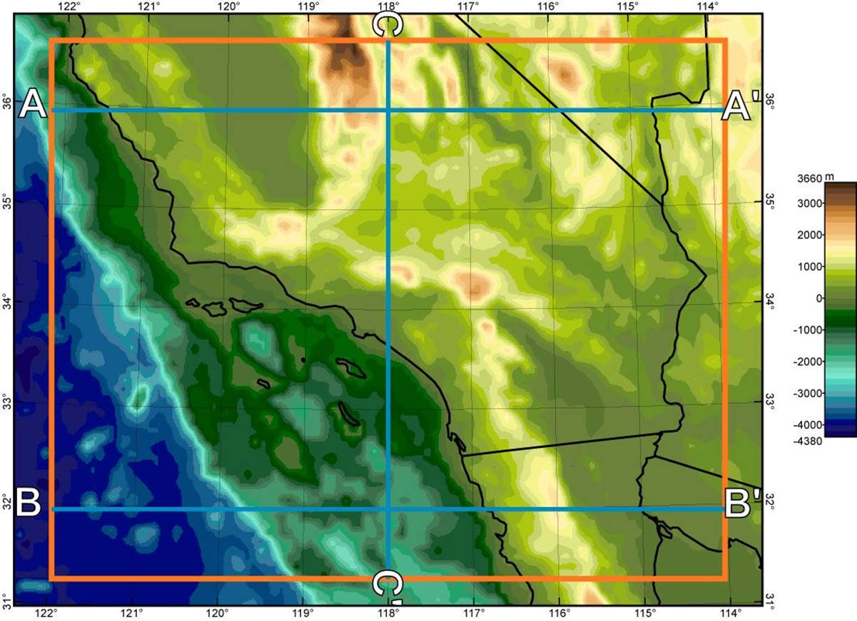
Figure 1. Location of the model region (brown box) and of 3 vertical sections (blue lines) shown below in Figure 10. Colored map shows topography/bathymetry from the ETOPO5 DEM (with 5’ resolution) used in the calculation. Coastlines and state lines are indicated in black.
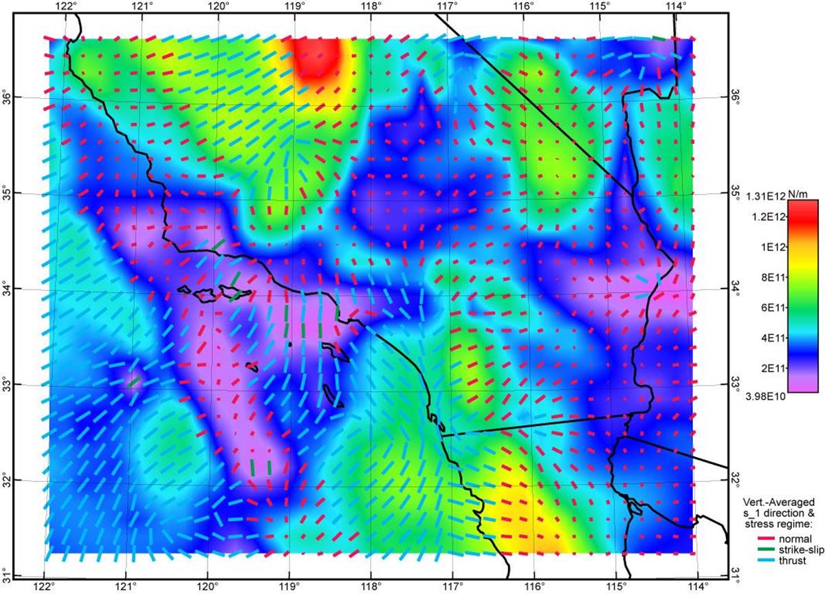
Figure 2. Topographic stress anomaly field computed from the seismic Moho model of Tape et al. [2012] and the ETOPO5 DEM (Figure 1) using assumed Poisson ratio of 0.25. Background color field shows the vertical integral of the greatest shear stress, in units of N m-1. Overlaid line segments show the trends of most-compressive principal topographic stresses; shorter line segments are foreshortened to suggest the plunges of these directions. Color of each line segment shows the dominant stress regime. Because this is an incomplete model that lacks any tectonic stress anomaly, its misfits to data are very large (see Table 1, row “Seismic0.25”).
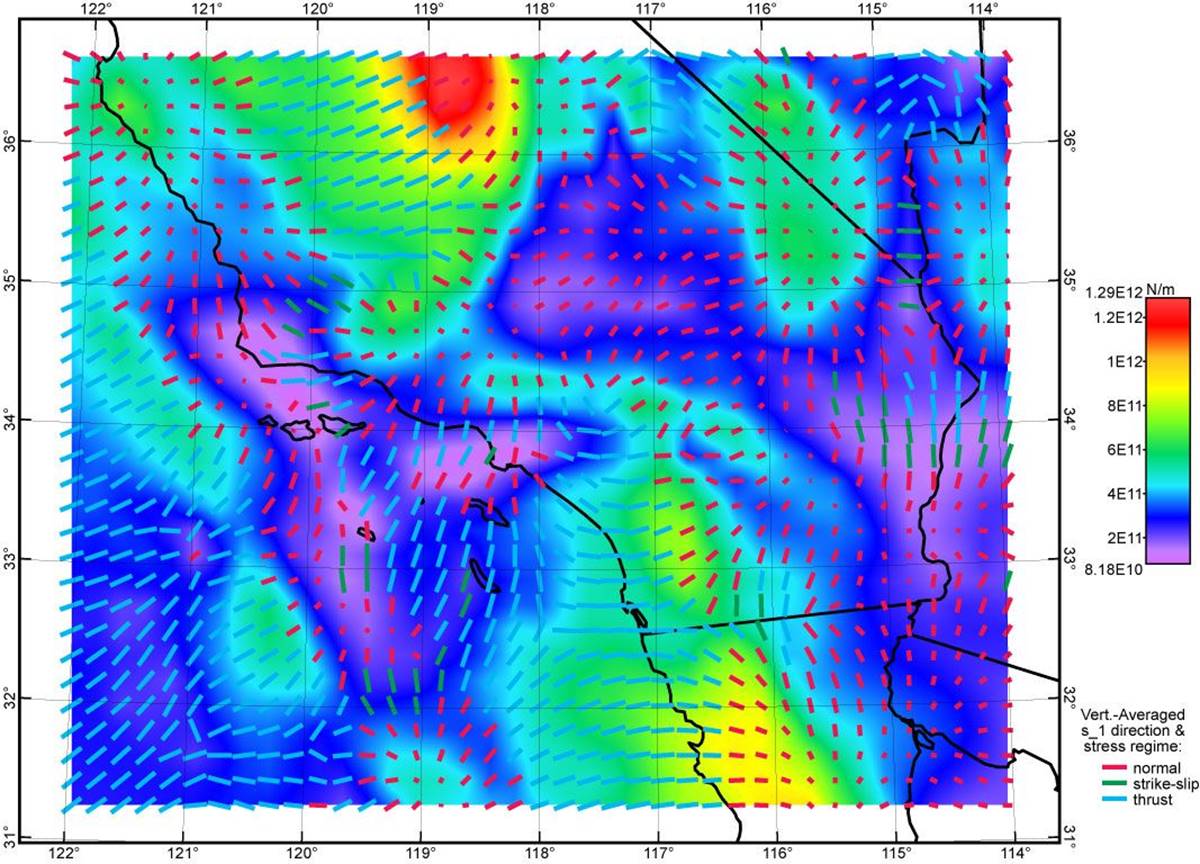
Figure 3. Topographic stress anomaly field computed from the seismic Moho model of Tape et al. [2012] and the ETOPO5 DEM (Figure 1) using assumed Poisson ratio of 0.50. Graphical conventions as in Figure 2 above. Figures 2~5 use the same color scale. Because this is an incomplete model that lacks any tectonic stress anomaly, its misfits to data are very large (see Table 1, row “Seismic0.50”).
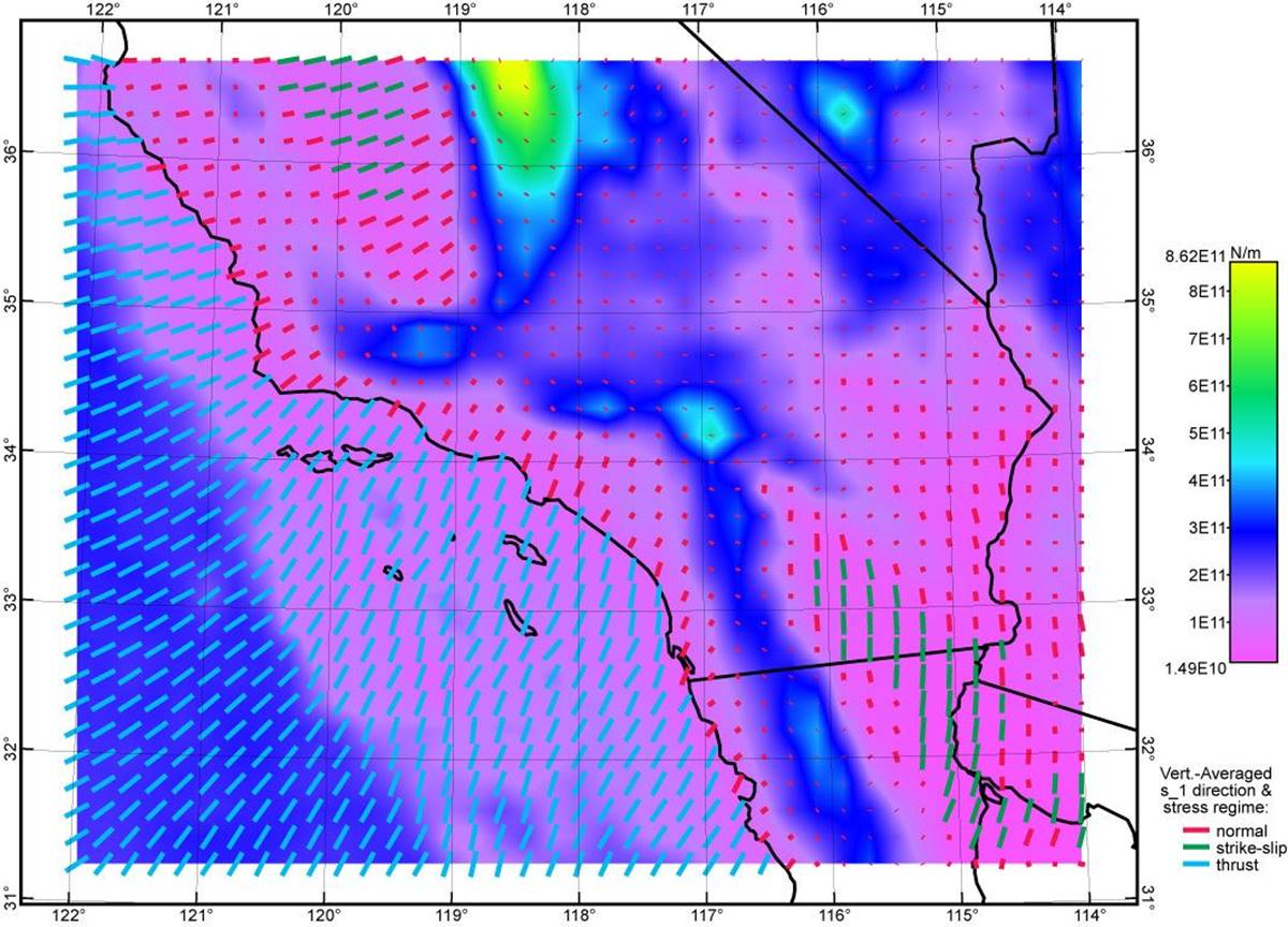
Figure 4. Topographic stress anomaly field computed from the isostatic Moho model of this paper and the ETOPO5 DEM (Figure 1) using assumed Poisson ratio of 0.25. Graphical conventions as in Figure 2 above. Figures 2~5 use the same color scale. Because this is an incomplete model that lacks any tectonic stress anomaly, its misfits to data are very large (see Table 1, row “Isostasy0.25”).
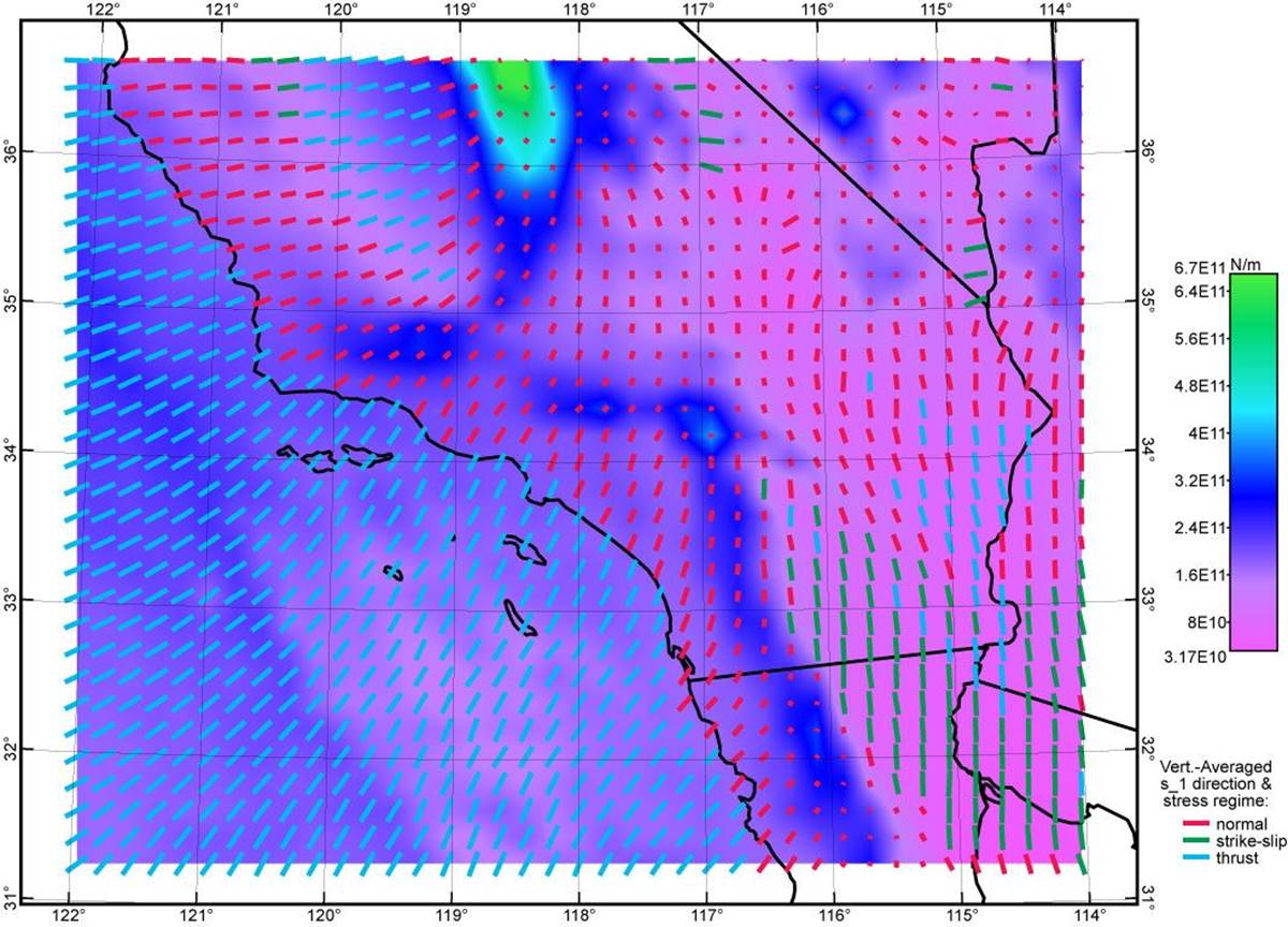
Figure 5. Topographic stress anomaly field computed from the isostatic Moho model of this paper and the ETOPO5 DEM (Figure 1) using assumed Poisson ratio of 0.50. Graphical conventions as in Figure 2 above. Figures 2~5 use the same color scale. Because this is an incomplete model that lacks any tectonic stress anomaly, its misfits to data are very large (see Table 1, row “Isostasy0.50”).
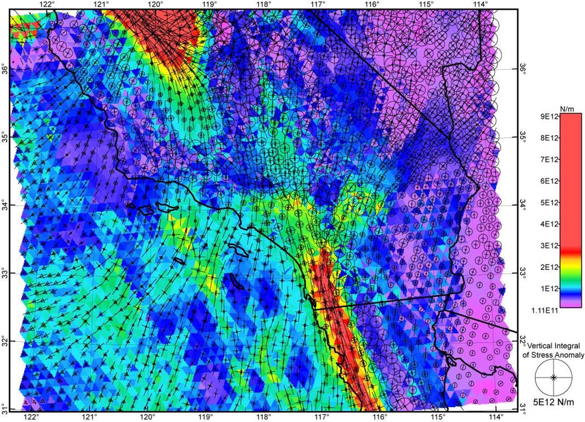
Figure 6. Vertically-integrated shear stresses (colors) and vertically-integrated stress anomaly tensors (discrete symbols with horizontal paired-arrows, and circle or triangle for the vertical component), according to the dynamic F-E model of southern California CSM2013001 computed with Shells. Deviatoric stresses from this model (which is also in the CSM library at SCEC) were used as target values for the FlatMaxwell solutions.
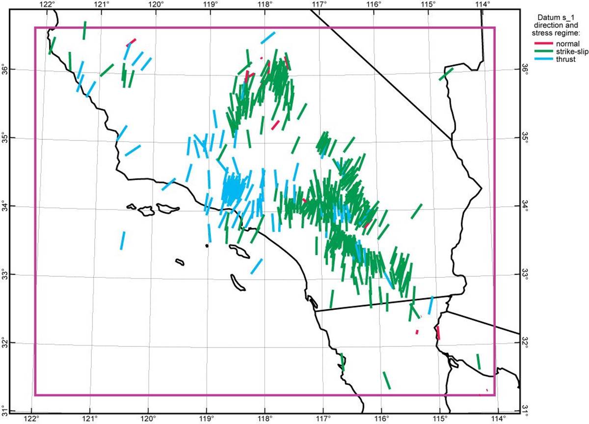
Figure 7. Most-compressive principal stress azimuths (449 line segments) with stress regimes (line color) obtained from the World Stress Map release of 2008 [Heidbach et al., 2008]. Shorter lines indicate plunging compression directions which are foreshortened. Most of these are obtained from earthquake focal mechanisms, but a small minority are from borehole observations. These principal stress directions (and stress intensities, where known) are also used as targets for the FlatMaxwell solutions.
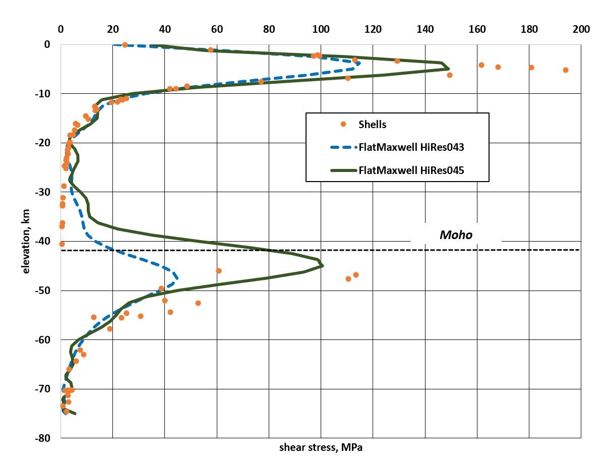
Figure 8. Vertical profiles of target shear stresses from the Shells model (dots) and the resulting vertical profiles of shear stress in two FlatMaxwell solutions (curved lines). This comparison uses a location (116.6°W, 32°N) within the western slope of the Peninsular Ranges of southwestern California where heat-flow is low [Blackwell & Steele, 1992] and shear stresses are high. Note that model HiRes043 tends to under-fit the higher shear stresses, while model HiRes045 comes closer to representing them. On the other hand, model HiRes043 has less unphysical “ringing” of shear stress estimates in weak layers. Both models illustrate the difficulty that the FlatMaxwell model has in fitting discontinuities in horizontal compression (and therefore, in greatest shear stress) across the Moho (here, at depth of 42 km).
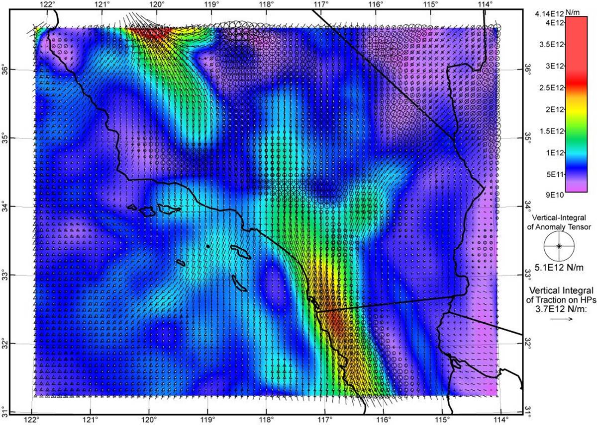
Figure 9. Vertically-integrated shear stresses (colored map) from FlatMaxwell model HiRes045, which was based on topographic stress model Isostasy0.50, with equal weight on the Shells and WSM target stresses. Overlain tensor symbols also represent vertically-integrated stress anomaly.
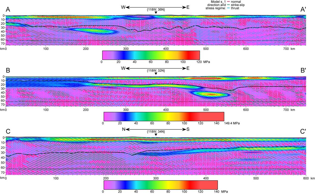
Figure 10. Three vertical sections (at locations shown in Figure 1) through model HiRes045 (of Figure 9), which was based on topographic stress model Isostasy0.50, with equal weight on the Shells and WSM target stresses. Colors show amplitude of the greatest shear stress (on any plane) at points in the plane of section. Overlain line segments show orientations of the most-compressive principal stress axis; shorter line segments imply an orientation more nearly normal to the section which is foreshortened. Color of the overlaid line segment indicates tectonic regime (normal, strike-slip, thrust). Moho is shown with solid black line. Topography and bathymetry are shown with no vertical exaggeration.