You need at least two gridded data files, one for elevation, and one for heat-flow. Each should give values at points on a regular rectangular grid in (longitude, latitude) space. You must use the (longitude, latitude) variant of the gridded data (.grd) file format. (However, it is not necessary for the two grids to have the same shape or grid spacing, as long as each grid covers your whole finite element model.) If you want to create your own .grd files, this step will require some light programming, in the language of your choice. However, it is possible that you will be able to use the files I have provided, in folders /oldFTP/neotec/Shells/Earth2/global_GRDs/ and /oldFTP/neotec/Shells/Earth5/global_GRDs/.
Positive values should be used for elevations above sea level, and negative values for bathymetry below sea level. The most convenient source of elevation/bathymetry is the ETOPO5 data set provided by the NOAA National Data Centers. (The newer GLOBE data set has higher resolution, but does not include water depths.) An example of ETOPO5 data was previously seen in Step 1. I advise using units of meters, consistent with use of SI units for all other quantities in this modeling project.
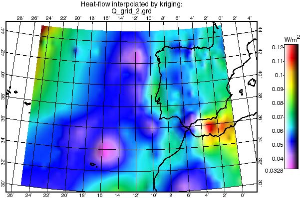
I advise using SI units of W/m2 (NOT mW/m2), consistent with SI units for other quantities in this modeling project. Heat-flow is only available from wells of convenience, so it cannot be measured on a regular grid and must be interpolated (or spatially averaged) to produce one. A global compilation of heat-flow data was provided by Pollack et al. (1991) and described in the journal article by Pollack et al. (1993; J. Geophys. Res., v. 98, #B7, 12,207-12,218). The most elegant method of interpolation is kriging (because it makes use of the statistical properties of the data), but this is not the place for a course on the subject. Spatial averaging with 1/r2 weighting often gives reasonable results as well. It is desirable to exclude extremely high values taken at volcanoes, as these are subject to a strong sampling bias! An example of a heat-flow map produced by kriging interpolation is seen below.
If you want to produce "generic" models which have no variations in topography or heat-flow, you can do so very quickly. By hand, type dummy .grd files with 4 equal values at the corners of one very large cell. For example, to impose constant elevation of 50 m and constant heat-flow of 0.054 mW/m2 in the region 18-30ºE, 15-25ºN, use:
elevation.grd:
|
|
heatflow.grd:
|
|
It is advisable to plot your .grd files to check for errors and problems. The plot below was produced by my program FiniteMap. Another option is to plot with my older graphical program OrbMapAI.
