58. Bird, P. [2009] Long-term fault slip rates, distributed deformation rates, and forecast of seismicity in the western United States from joint fitting of community geologic, geodetic, and stress direction data sets, J. Geophys. Res., 114(B11), B11403, doi:10.1029/2009JB006317, with electronic supplements.

ABSTRACT.  The long-term-average velocity field of the western United States is computed with a kinematic finite-element code.  Community datasets include fault traces, geologic offset rates, geodetic velocities, principal stress directions, and Euler poles.  There is an irreducible minimum amount of distributed permanent deformation, which accommodates 1/3 of Pacific-North America relative motion in California.  Much of this may be due to slip on faults not included in the model.  All datasets are fit at a common RMS level of 1.8 datum standard deviations.  Experiments with alternate weights, fault sets, and Euler poles define a suite of acceptable community models.  In pseudo-prospective tests, fault offset rates are compared to 126 additional published rates not used in the computation: 44% are consistent; another 48% have discrepancies under 1 mm/a, and 8% have larger discrepancies.  Updated models are then computed.  Novel predictions include: dextral slip at 2~3 mm/a in the Brothers fault zone, two alternative solutions for the Mendocino triple junction, slower slip on some trains of the San Andreas fault than in recent hazard models, and clockwise rotation of some domains in the Eastern California shear zone.  Long-term seismicity is computed by assigning each fault and finite element the seismicity parameters (coupled thickness, corner magnitude, and spectral slope) of the most comparable type of plate boundary.  This long-term seismicity forecast is retrospectively compared to instrumental seismicity.  The western U.S. has been 37% below its long-term-average seismicity during 1977-2008, primarily because of (temporary) reduced activity in the Cascadia subduction zone and San Andreas fault system.

P.S. This proposal that “distributed permanent deformation … accommodates 1/3 of Pacific-North America relative motion in California” was surprising at the time.  However, similar fractions (ranging from 27% to 38%) have been obtained in a number of other neotectonic-modeling studies: Parsons et al. [2013, USGS OFR 2013-1165], Johnson et al. [2013, J.Geophys. Res.], Zeng & Shen [2016, BSSA]; and Hearn [2019, Tectonophysics].
{Note added 2019.03.20 by PB; thanks to Liz Hearn for this tidy summary!}

final manuscript with tables and figures

neotectonic finite-element program NeoKinema  [N.B. Latest version, improved from that in electronic supplement.]

graphical program NeoKineMap  [N.B. Latest version, improved from that in electronic supplement.]

input and output datasets for preferred NeoKinema model GCN2008088

gridded long-term seismicity forecast from preferred model GCN2008088 and program Long_Term_Seismicity_v3

Figures

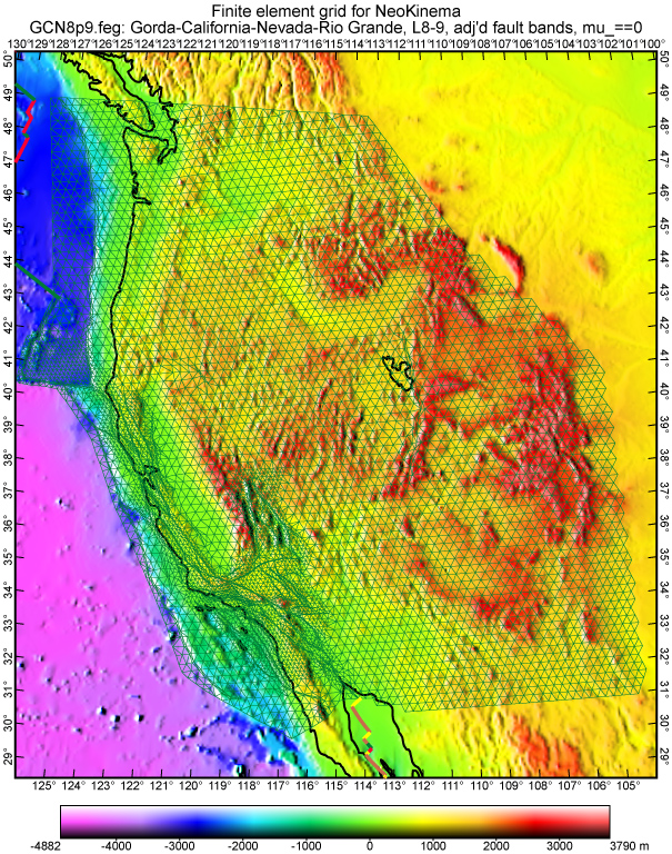
Figure 1.  Finite element grid GCN8p9.feg used in this study.  Most of the grid is composed of quasi-equilateral spherical triangles, with sides of either 30 km (coarse regions) or 15 km (fine regions).  Ribbons of smaller elements, with width approximately 4 km, have been inserted along most fast-slipping faults to better approximate the expected velocity discontinuities.  There are 6452 nodes and 12627 elements.

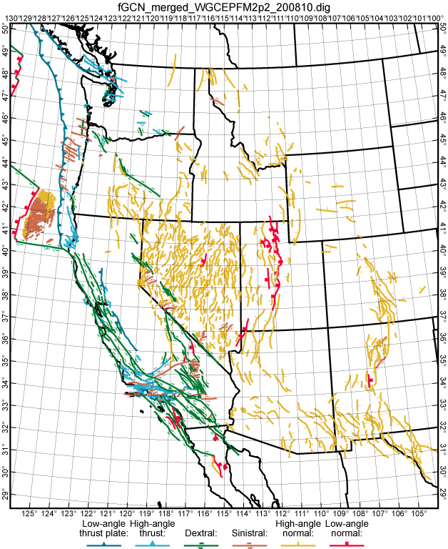
Figure 2.  Traces of 1472 active and potentially-active faults included in these models.  Traces are colored according to prior expectations of their predominant sense(s) of slip.  Faults with oblique slip have a green or brown trace to indicate dextral or sinistral component, plus dip-ticks of a different color and shape to indicate the primary mode of dip-slip.  Offset type D is used for both low-angle detachment faults and magmatic spreading centers.

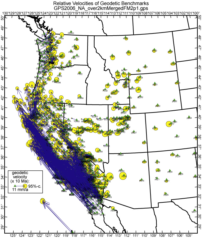
Figure 3. GPS benchmarks, interseismic velocities, and 95%-confidence ellipses used in modeling.  As described in text, California velocities are from a 2006 solution by Shen and others for WGCEP; velocities outside California are selected from the PBO solution of September 2007.  All velocities are in the stable North America reference frame.  Guadalupe Island is just visible at the southern margin of the map.

.

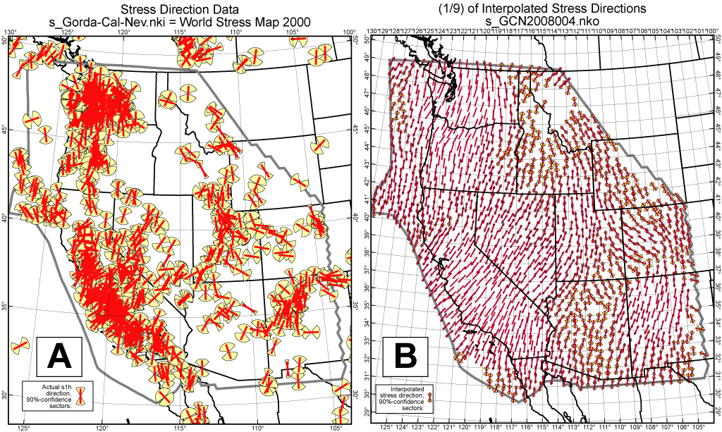
Figure 4.  Data on the azimuth of the most-compressive horizontal principal stress from the World Stress Map (A), and directions interpolated by NeoKinema (B) using the clustered-data algorithm of Bird & Li [1996].

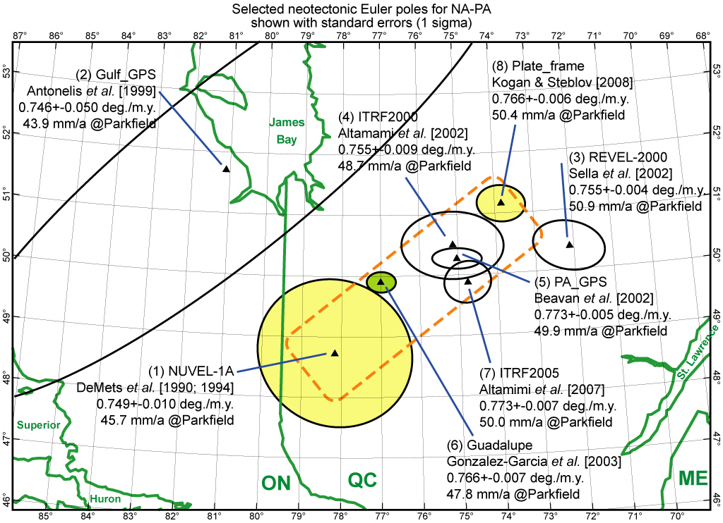
Figure 5.  Neotectonic Euler poles for relative rotation of North America (NA) with respect to Pacific (PA).  The error ellipses shown are standard errors, so 95%-confidence ranges have twice the diameters shown, and typically overlap.  For each pole, a label indicates the implied NA-PA relative velocity at Parkfield, CA (assuming that stable NA and PA lithosphere extend up to the San Andreas fault at that point, whereas actually they do not).  Poles within the dashed rectangle were used in NeoKinema modeling; others are shown for historical interest.  The Gulf_GPS pole was not explicitly stated by Antonelis et al. [1999] but was computed by the author from their velocity vectors.

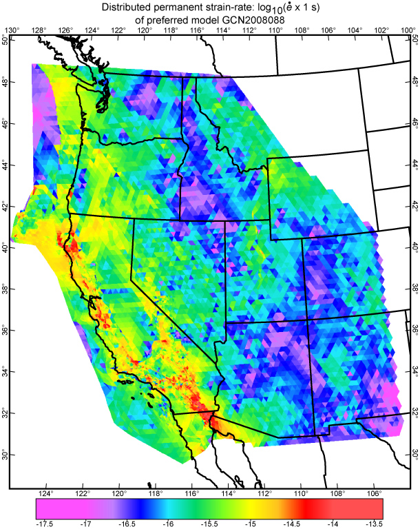
Figure 6. Common logarithms of distributed permanent strain-rates (excluding strain-rates due to slip on modeled faults) in the preferred model GCN2008088.  See equation (5) for definition of scalar measure .

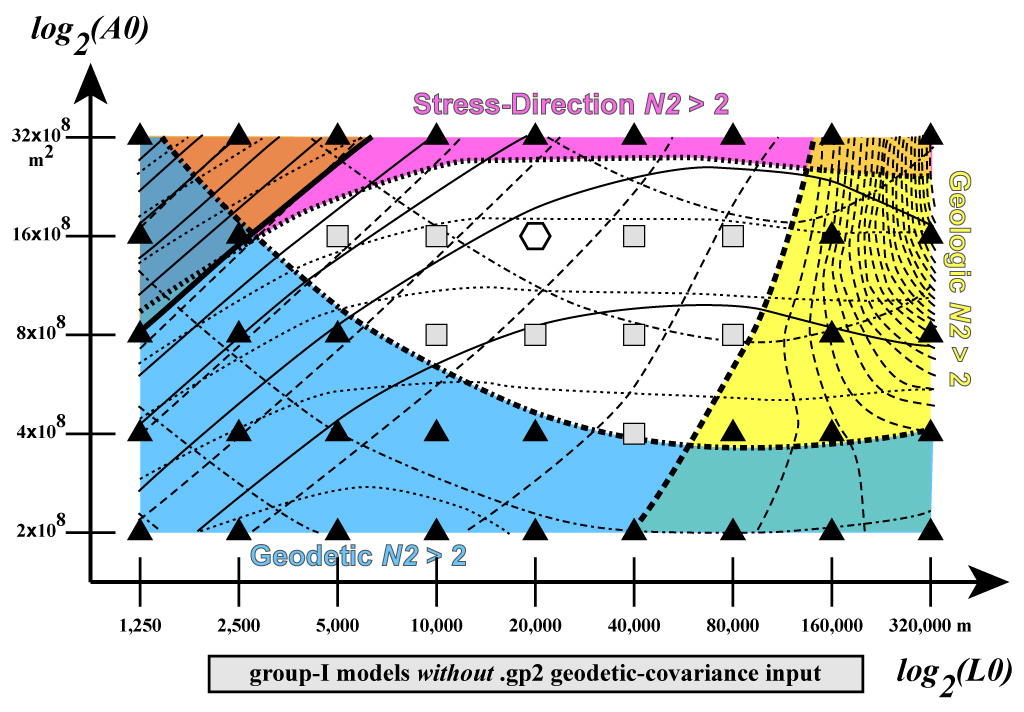
Figure 7.  Three misfit measures (, , ) are contoured in a 2-D parameter space with axes of  and .  Contour interval 0.2, with heavier lines at value 2.0, and colored shading to show regions of unacceptable misfit (any ).  Acceptable models are shown by rectangles and octagon, while unacceptable models are shown by triangles.  All computations used prior/input , Fault Model 2.1, NUVEL-1A pole, and block-diagonal approximation of the geodetic covariance.

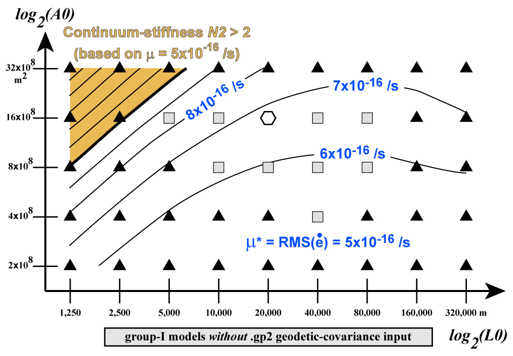
Figure 8.  Posterior/output values of RMS distributed permanent strain-rate () shown with contours in the same 2-D parameter space as Figure 7.  All inputs as in Figure 7.  Acceptable models (with all misfit measures < 2) are shown by rectangles and octagon, while unacceptable models are shown by triangles.

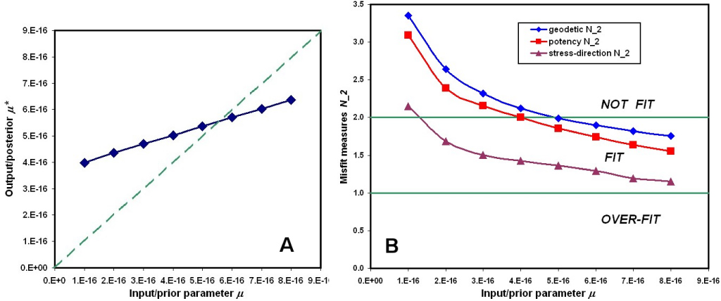
Figure 9.  Posterior/output values of RMS distributed deformation rate (, in A) and 3 misfit measures (, , , in B) plotted as functions of input parameter , with fixed weights (=4×10⁴ m, =4×10⁸ m²), and other inputs as in Figure 7.  Note that output  is relatively insensitive to input , and that this problem has a natural minimum  of 5×10^-16 /s.

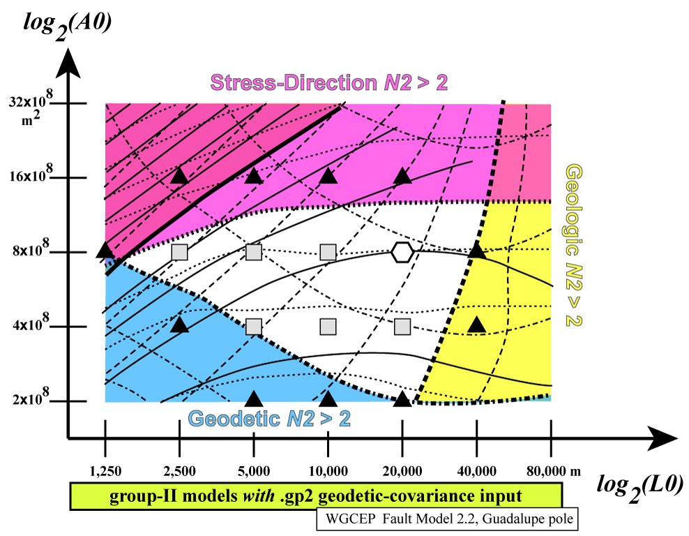
Figure 10.  Three misfit measures (, , ) are contoured in a 2-D parameter space with axes of  and .  All conventions as in Figure 7.  The differences here are that the full covariance matrix of California GPS velocities is used, the NA-PA Euler pole is the Guadalupe pole, and southern California fault traces are from WGCEP Fault Model 2.2.

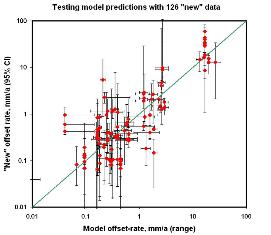
Figure 11.  A pseudo-prospective test of the ability of the set of 16 successful “community” models to predict “new” long-term geologic offset rates which were not used in their computation.  Data sources in Table 4.  Large discrepancies are discussed individually in text Section 7.

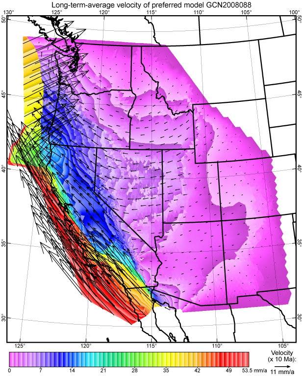
Figure 12.  Long-term velocity field of the preferred model GCN2008088.  Note that effects of transient elastic strain accumulation about the Cascadia trench and San Andreas fault system (and all other faults) have been removed.  Brightness contour interval 1 mm/a; jagged contours are caused by velocity discontinuities across faults.  For legibility, velocity vectors are shown at only 1/9 of nodes.  Velocity reference frame is stable eastern North America.

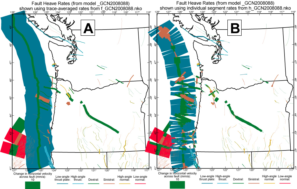
Figure 13.  Fault heave rates from preferred model GCN2008088 in the Washington-Oregon region, displayed in two formats: (A) The trace-averaged heave rate is plotted at every point along the trace, giving ribbons of uniform width.  (Oblique slip is represented by two ribbons of different colors plotted along the same trace.)  (B) Individual per-element heave rates are plotted, without enforcing continuity along trace.  This “noisy” plot has the potential advantage of displaying predicted variations in offset rate along each trace.  However, it also displays probable artifacts, such as implausible high rates in elements where faults terminate without any fault junction.

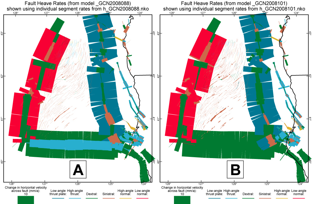
Figure 14.  Fault heave rates predicted by NeoKinema in the region of the Mendocino triple junction.  (A) Preferred model GCN2008088, in which the Mendocino fault is allowed to slip obliquely and absorbs 10 mm/a of N-S shortening by underthusting Gorda crust under Pacific.  (B) Ad-hoc model GCN2008101 in which the Mendocino fault is vertical, and shortening takes place by distributed deformation, faster sinistral faulting within the Gorda crust, and its accelerated subduction at the south end of the Cascadia trench.

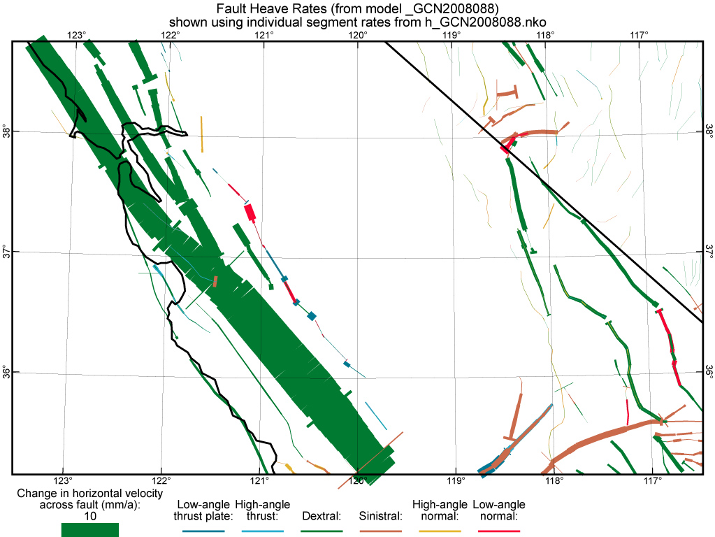
Figure 15.  Fault heave rates from preferred model GCN2008088 in the San Francisco Bay, central California Coast Ranges, and central and southern Walker Lane regions.

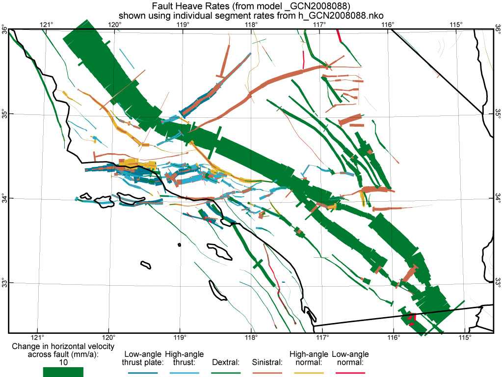
Figure 16.  Fault heave rates from preferred model GCN2008088 in southern California.

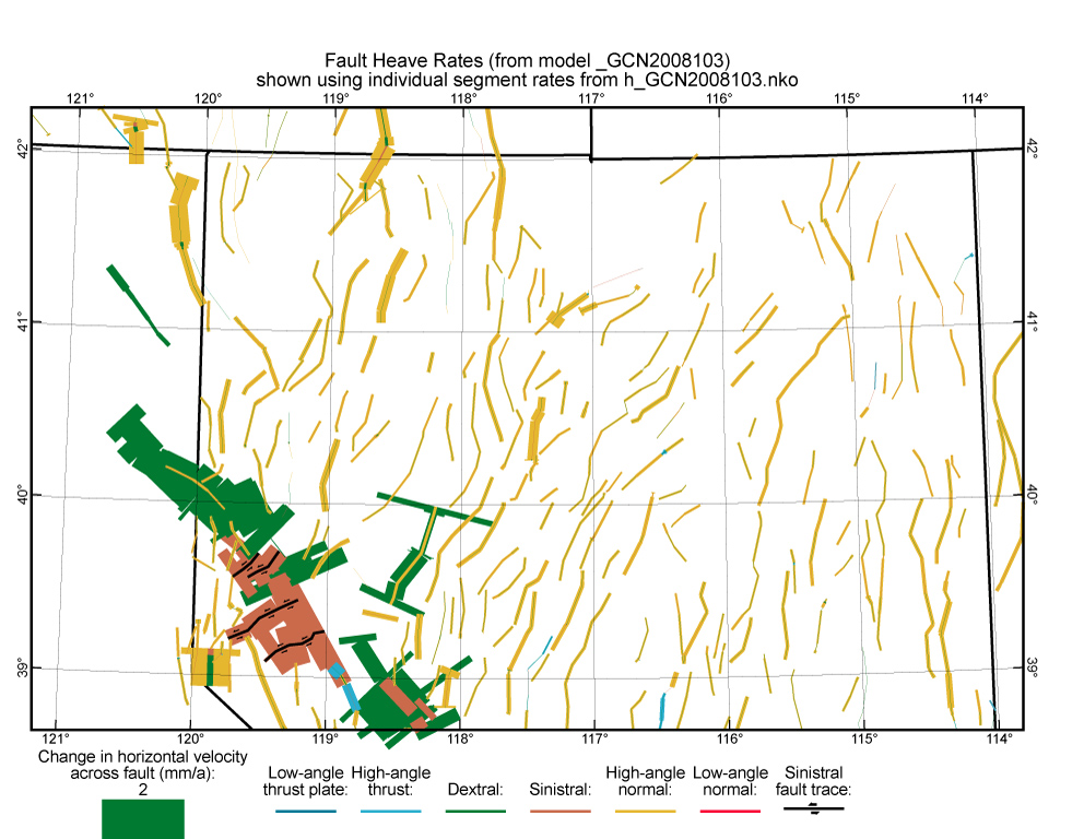
Figure 17.  Fault heave rates from model GCN2008103 in the northern Walker Lane and northern Nevada.  In the Walker Lane, fault traces have been overlain on the heave-rate ribbons of 4 NE-trending sinistral faults.  Elsewhere, fault traces are not overlain because they would obscure small heave-rates.

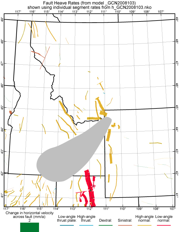
Figure 18.  Fault heave rates from model GCN2008103 in the northern Rocky Mountains and northeastern Basin & Range province.  While few faults are mapped within the Snake River Plain (shaded), it is moving [Payne et al., 2008] and deforming by other means [Parsons et al., 1998].

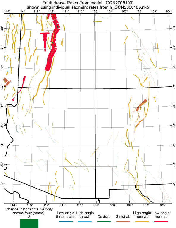
Figure 19.  Fault heave rates from model GCN2008103 in the regions surrounding the Colorado Plateau.

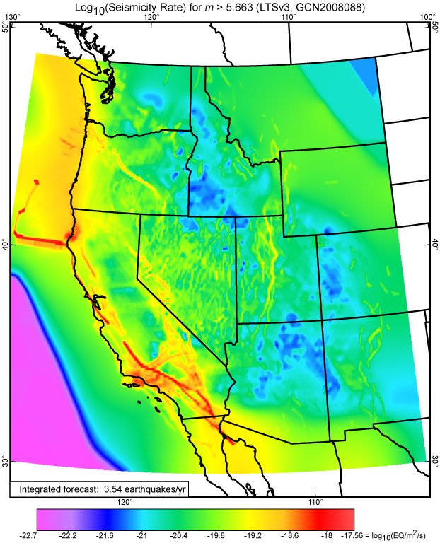
Figure 20. Common logarithm of long-term shallow seismicity (epicenters per square meter per second, including aftershocks) for threshold magnitude 5.663 (moment 3.5×10¹⁷ N m), computed by Long_Term_Seismicity (v.3) from preferred NeoKinema model GCN2008088.  Seismicity around the margins, outside the NeoKinema model domain, is based on relative plate motions from model PB2002 of Bird [2003] and intraplate strain rates from dynamic Shells model Earth5-049 of Bird et al. [2008].  Rates in central Montana and eastern Wyoming are too high, for reasons explained in that paper.  The spatial integral of these forecast rates is 113 earthquakes per 31.92 years in the depth range 0~70 km.  (To convert seismicity from earthquakes/m²/s to earthquakes/km²/year, add 13.5 to the values along the logarithmic scale.  To convert to earthquakes/(100 km)²/century, add 19.5.)

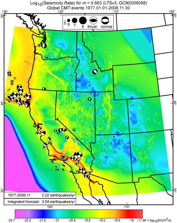
Figure 21. Colored background shows long-term forecast, exactly as in Fig. 20.  For retrospective comparison, the Harvard CMT catalog shows 71 events (with focal mechanisms on lower focal hemispheres) of m>5.663 at 0~70 km depth in the 31.92-year interval 1977.01.01~2008.11.30.  This figure illustrates why the instrumental record of seismicity is very inadequate for estimating maps of long-term seismicity.