![]()
![]()
![]()
![]()
![]()
Step 8: Plot the fault-traces map with NeoKineMap
It is time to get acquainted with my associated map-making utility program NeoKineMap.
Even in advance of any NeoKinema solution, you can use it to check (and
publish) many aspects of your input data.
We will begin here by making an elegant map of the fault traces that you have
been working on in previous steps.
Aside: Many runs of NeoKineMap will eventually ask you
for the name of your parameter-file (p_*.nki)
most recently used with NeoKinema?
(It will then read this parameter file to obtain the names of all other input
and output files. This reduces typing, and also reduces careless errors.)
Since you do not yet have your own, customized version of these parameters,
begin with a “generic” set of parameters,
as provided in file parameters_for_NeoKinema.nki.txt.
(Remember to remove the “.txt”
filename-extension from this file-name after you download it.)
_test01
[name token for this run of NeoKinema; anything you like!]
2.00E4 L0 = length of fault trace
whose offset rate gets unit weight (in m)
8.00E8 A0 = area of continuum whose
stiffness & isotropy get unit weight (in m**2)
40
refinements (for nonlinearity) allowed in this solution (try 20-40)
5.0E-16 mu_ = scalar measure of typical
anelastic strain rates in continuum (/s)
1.0E-17 xi_ = small strain-rate increment,
in /s (Not TOO small! Suggestions: 1.0E-17 to 1.0E-20 /s.)
20. sigma, in
degrees, of angle between [heave vectors of dip-slip faults] &
[trace-normal direction]
6371. radius of planet, in
kilometers
1. 12. minimum and maximum default
locking depths of intraplate faults, in km (may be overridden by f*.nki)
14. 40. minimum and maximum default locking
depths of subduction zones, in km (may be overridden by f*.nki)
FALSE switch: Do active faults
give sigma_1h direction data?
f_test01.nki filename of fault offset-rates (or, 'none')
f_test01.dig filename of digitized
fault traces (or, 'none')
s_test01.nki filename of horizontal principal stress directions (or,
'none')
1
stress interpolation method: (1) Bird & Li [1996]; (2) Carafa & Barba
[2013].
WUSC002.gps filename of geodetic velocity data (or, 'none')
WUSC002.gp2 filename of covariance matrix for geodetic velocity
components (or, 'none')
FALSE switch: Is the reference
frame of geodetic-velocity data allowed to free-float?
FALSE
conservative_geodetic_adjustment? (uses geologic slip rates; not
self-consistent)
test01.feg filename of finite element grid (required)
b_test01.nki filename of boundary conditions for finite element grid
(required)
NA plate
defining velocity reference frame for type-4 boundary conditions
FALSE dump_all_solutions?
Creates velocity log file for studying convergence.
You can edit this parameter.nki
file in any plain-ASCII text editor, such as NotePad or EditPad Pro.
Right now, the only thing you need to do is replace the name “f_test01.dig”
with the actual name of your digitized fault traces file.
After that, you can save the (revised) parameter file under any filename you
prefer (but it should end with “.nki”).
Also, remember that NeoKineMap will require the “generic template”
file AI7frame.ai to be present (and accessible)
on your computer.
You can just copy this from my web site; you will not need to modify it.
Keep a copy of this file in the “home folder” where file NeoKineMap-WinNNseq.exe
is saved, and started. (Note: NN = 32 or 64)
After some introductory lines, and some questions about your preferred input
& output paths (e.g., path to your Desktop?),
NeoKineMap will ask you for a name for the Adobe Illustrator .ai file that you will
create in this run.
You can choose any filename you like, as long as it ends with .ai
When NeoKineMap asks you for the size of the paper on which the map
will be created, one logical choice would be to describe the size of the paper
currently in your printer.
For example, in America I would specify width 8.5” and height 11” (for portrait-format)
or width 11” and height 8.5” (for landscape-format).
A landscape format of about this size is also a good choice for any map that
will end up as a PowerPoint slide, later on.
Alternatively, you can specify a really large piece of “virtual paper” even
though you have no realistic hope of printing it.
I sometimes specify a map-page as large as my digitizing tablet (36” × 24” in
American inches).
Even if a really large plot like this can only be examined inside Adobe
Illustrator, you can scan and zoom easily there,
both zooming-out to see the whole fault network, and zooming-in to read the
“F1234R” fault-trace-index numbers.
When NeoKineMap asks you for the map-projection you want, you could
choose to use the same map-projection that you previously described to Projector.
Or, you could switch to a completely different projection and/or scale.
When NeoKineMap offers to plot a (colored-area) “Mosaic” layer, decline this offer, with “No”.
When NeoKineMap offers a choice of (line-based) “Overlay” layers, a
good starting choice is:
1 :: digitized basemap
(lines-type)
because this gives you the chance to plot your file of
coastlines/state-lines/border-lines, in (longitude, latitude)
coordinates, that you created earlier.
Or, if you don’t have such a file, perhaps you could use North_America_states.dig
or WorldMap.dig which are posted on my
web site.)
When NeoKineMap asks, “Do you want additional overlays?” answer
“Yes”.
Then select overlay type of:
4 :: fault traces
and then enter the name of your digitized-fault-traces file, in (longitude,
latitude) coordinates, ending with “.dig”.
After NeoKineMap asks a few final questions about the longitude/latitude
graticule you want, and any map titles,
it will exit and leave behind a new Adobe Illustrator .ai file.
Open this new file in Adobe Illustrator, and you should see something like the map below (but, using your data):
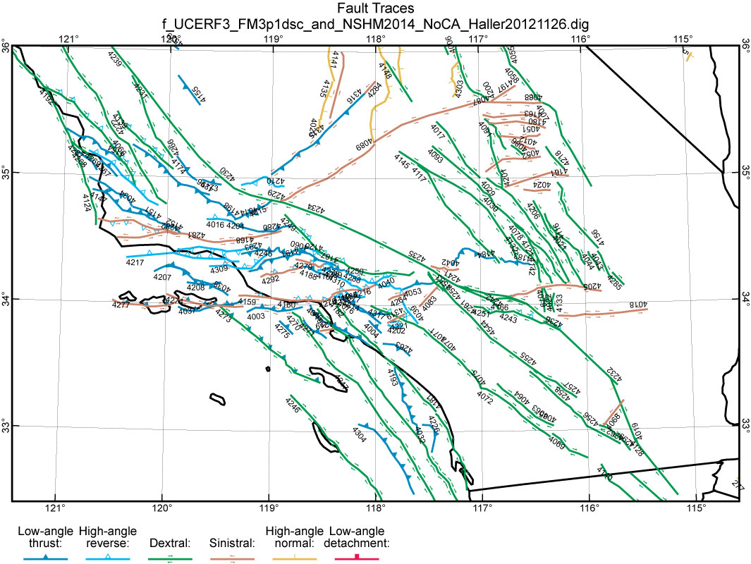
If you use the black-arrow Selection Tool in Adobe Illustrator to click on one of the fault trace numbers, the whole group of numbers will be selected. Then, you have the option to do Object / Hide / Selection to make a prettier map (but, without deleting this essential information).
Among the powerful options now available to you are to use Adobe
Illustrator to File / Save As:
.PDF,
or to File / Save for Web & Devices: creating bitmap versions in
either .JPG or .GIF format.
Another cool Adobe Illustrator trick is to use Edit / Find and
Replace… to locate any “lost” fault-trace by its Fnnnn
index number.
Just type this integer index number into the search box (leaving out the “F”, and also leaving out any
leading zeros) and press “Find”.
If this index number is anywhere on the map, Adobe Illustrator will highlight
it (and perhaps scan over to it).
(Just one caution: If you type the number and then type “Enter” this AI
command does not work(!). You must use your mouse to press the “Find”
button.)
As you examine your new fault-trace map for errors (such as omitted fault
traces), you may notice that one or more faults are dipping the wrong way.
This happens when a fault trace was digitized in the wrong direction, which
usually happens when you accidentally wrote the fault-trace index-number at the
wrong end of the trace.
There are 3 ways to correct any faults that dip the wrong way:
1. Run my utility program ReverseDIG, which goes through the traces one-by-one, shows you their header lines (and some geometric information), and then asks whether this trace should be reversed?
2. Use a plain-ASCII text editor (such as NotePad or EditPad Pro) to manually reverse the order of the (lon, lat) points within the bad fault trace(s) in your .dig file.
3. Re-digitize the bad trace(s) in (x, y) coordinates [Step 4] and use Projector again to convert to (lon, lat) [Step 5]; then use a plain-ASCII text editor to replace the bad polyline(s) in your fault-traces .dig file.
Usually method (1) above is the fastest and most error-free.
![]()
![]()
![]()
![]()
![]()