61. Bird, P., C. Kreemer, and W. E. Holt [2010] A long-term forecast of shallow seismicity based on the Global Strain Rate Map, Seismol. Res. Lett., 81(2), 184-194, doi: 10.1785/gssrl.81.2.184.
Introduction. The Global Strain Rate Map (GSRM) of Kreemer et al. (2003) was the main result of Project II-8 of the International Lithosphere Program. The GSRM is a numerical velocity gradient tensor field model for the entire Earth’s surface that describes the spatial variations of horizontal strain rate tensor components, rotation rates and velocities. The model consists of 25 rigid spherical plates and ~25,000 0.6° by 0.5° deformable grid areas within the diffuse plate boundary zones (e.g., western North America, central Asia, Alpine-Himalaya belt). The model provides an estimate of the horizontal strain rates in diffuse plate boundary zones as well as the motions of the spherical caps . This is one of the first successful models of its kind that includes the kinematics of plate boundary zones in the description of global plate kinematics.
The vast majority of the data used to obtain the GSRM comes from horizontal velocity measurements obtained using Global Positioning System (GPS) measurements. The latest model version of May 2004 (i.e., GSRM v.1.2) includes 5170 velocities for 4214 sites world-wide (Holt et al., 2005). Most geodetic velocities are measured within plate boundary zones. The observed velocities are obtained from 86 different (mostly published) studies. The model includes additional constraints on the style (not magnitude) of the strain rate tensor inferred from moment tensors of shallow earthquakes. In addition, geologic strain rates in central Asia inferred from Quaternary faulting data are fit simultaneously with the geodetic velocities to improve the model there. See Kreemer et al. (2000; 2003) for more details.
It was always a goal of the GSRM Project to support long-term forecasts of seismicity based on tectonic deformation. Two recent developments make this especially timely. First, the Collaboratory for the Study of Earthquake Predictability (CSEP; Jordan et al. 2007) is accepting global models for prospective testing. To date, they have only registered global models that are based on smoothing of instrumental seismicity (e.g., Kagan and Jackson 2010?), so it would be valuable to compare results with a model based on tectonics. Second, the Global Earthquake Model project will soon create an update to the Global Seismic Hazard Map of Giardini et al. (1999), which was based primarily on instrumental and historical catalogs. The new map is likely to be based primarily on traces and slip rates of faults, so comparisons to seismicity models incorporating geodesy and plate tectonics should be illuminating and helpful.
To convert the GSRM to a forecast of long-term shallow seismicity, we apply the hypotheses, assumptions, and equations of Bird and Liu (2007), who referred to them as the Seismic Hazard Inferred From Tectonics (SHIFT) hypotheses: (1) The long-term seismic moment rate of any tectonic fault, or any large volume of permanently-deforming lithosphere, is approximately that computed using the coupled seismogenic thickness (i.e., the seismic coupling coefficient times the seismogenic thickness) of the most comparable type of plate boundary; and (2) The long-term rate of earthquakes generated along any tectonic fault, or within any large volume of permanently-deforming lithosphere, is approximately that computed from its moment rate (of the previous step) by using the frequency/magnitude distribution of the most comparable type of plate boundary.
In this conversion, we faced four conceptual and/or practical difficulties:
First, the strain-rates available are not always the kinds of strain-rates that would be preferred. The strain-rates in GSRM were largely determined by GPS geodetic velocities, assumed plate and boundary geometry, and some local geologic and strain-direction constraints. Except where faults are creeping (or where they have many small earthquakes during the measurement period), the strain-rates inferred from differentiation of GPS velocities are dominantly elastic strain-rates associated with rising deviatoric stresses. However, the strain-rates input to SHIFT calculations should ideally be long-term permanent strain-rates with no elastic components. Geodetic strain-rates typically have smoother map patterns than long-term permanent strain-rates which include singularities along fault traces. However, in a 2-D Earth-surface model based on plate-tectonic concepts, cross-boundary line integrals of these two kinds of strain-rate across a given plate boundary are the same, because both are equal to the relative plate velocity, regardless of timescale. The use of available GSRM strain-rates, which include some elastic components, should not greatly affect the total long-term seismicity computed in a SHIFT model, but only smooth its spatial distribution. On the scale of global maps and forecasts this smoothing is relatively insignificant compared to grid aliasing, digitization error, and other local error sources. Thus we disregard this distinction.
Second, GSRM treats plate interiors as perfectly rigid and predicts zero strain-rates in these regions. Yet a global seismicity forecast with zero rates in plate interiors would be both unrealistic and irresponsible. Our solution is to forecast a uniform low seismicity rate in all plate interiors, which is based on the collective frequency/magnitude distribution of these regions in the years covered by a reliable catalog. This makes our model formally a hybrid of two methods (SHIFT- and catalog-based), but as the two parts are spatially distinct there is little chance that these components will be confused.
Third, the basic SHIFT hypotheses do not specify how to decide which is the “most comparable type of plate boundary” for a given spatial grid point. This must be determined by subsidiary rules or hypotheses appropriate to the data and/or models available. We cannot use all of the decision rules suggested in Table 2 of Bird and Liu (2007) because they assumed that all subduction zones and spreading ridges were represented by discrete fault traces, which is not the case in GSRM. Fortunately, Kreemer et al. (2002) published a global map separating the deforming regions of GSRM into four deformation regimes: subduction, ridge/transform, diffuse oceanic, and continental (Figure 1). We use their map as the basis for assignments, and in some cases also use the tectonic style (e.g., normal-faulting, strike-slip, thrust-faulting, or mixed) of the local strain-rate tensor.
Finally, we found that our raw (uncorrected) forecast was seriously underpredicting global shallow seismicity (by a factor of 2) and that this was primarily due to underpredictions of subduction seismicity (by a factor greater than 3). We identified three quantifiable sources of underprediction in subduction zones: (1) inappropriate geometric factors in the moment-rate formula for many thrust faults whose dips are much less than 45°; (2) velocity-dependence of coupled seismogenic thickness in subduction zones inferred by Bird et al. (2009); and (3) time-dependence of global seismicity, which has increased since the calibration period of 1977-2002 studied by Bird and Kagan (2004). Compounding the corrections for these effects requires scaling-up the forecast seismicities of all grid points in the subduction-zone deformation regime by about a factor of 3. We apply smaller empirical correction factors to each of the other three deformation regimes. This yields an adjusted forecast that is reasonably consistent with the map-pattern and frequency/magnitude graph of the 33-year-old Global Centroid Moment Tensor catalog.
P.S. In December 2011, this model was installed in the Global testing region of the Collaboratory for the Study of Earthquake Predictability (CSEP). Specifically, it was placed in the high-resolution category (cell size 0.1 x 0.1 degree x 70 km) because our cell size of 0.6 x 0.5 degree x 70 km was not a good match for the low-resolution category (cell size 1 x 1 degree x 30 km). As of 2014.01, this testing had not yet started, and the test duration is undefined. Since our model does not include aftershocks or other time-dependent processes, we expect the model to do relatively better over longer time-windows (e.g., 10 years or more).
P.P.S. This tectonic forecast was updated in 2015 by using version 2.1 of the Global Strain Rate Map; please refer to Bird & Kreemer [2015a,b].
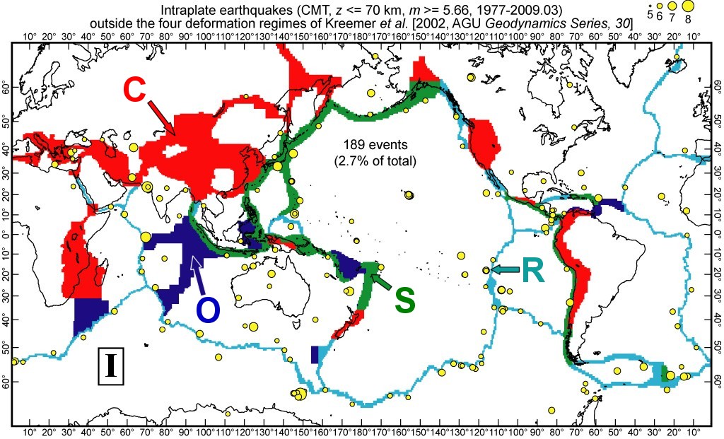
Figure 1.
Deformation regimes as defined by Kreemer et al.
(2002): Subduction (S); diffuse Oceanic (O); Ridge-transform (R); Continental
(C). Also shown are 189 shallow earthquakes above ![]() =
5.66 from the CMT catalog, 1977-2009.03, which did not fall into any of these
regimes. These are considered intraplate (I) earthquakes.
=
5.66 from the CMT catalog, 1977-2009.03, which did not fall into any of these
regimes. These are considered intraplate (I) earthquakes.
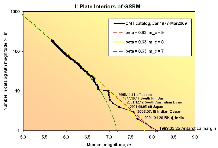
Figure 2. Frequency/magnitude plot of the 189 shallow intraplate earthquakes from Figure 1. Also shown are 3 tapered Gutenberg-Richter model curves (Jackson and Kagan, 1999; Kagan and Jackson, 2000). All models have the same asymptotic spectral slope of β = 0.63, but differ in the choice of corner magnitude mc. While the match to the curve with corner magnitude of 9 appears best, it must be noted that this depends on the size of the single largest earthquake.

Figure 3. SHIFT/GSRM global long-term forecast of the rates of shallow earthquakes above mT = 5.66. This model has been adjusted to match global shallow earthquake rates from CMT in 1977-2009.03 by using one free parameter for each of four deformation regimes, and one for the intraplate area. Rates are expressed as earthquakes per square meter per second, including aftershocks. Coloring of the map employs a logarithmic scale to express variations across almost 4 orders of magnitude from peak subduction-zone rates to intraplate rates. Mercator projection.
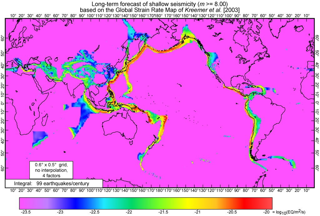
Figure 4. SHIFT/GSRM global long-term forecast of the rates of shallow earthquakes above mT = 8.00. Conventions as in Figure 3. In this model, mid-ocean spreading ridges and ideal oceanic transforms do not contribute to seismicity at magnitudes above 8, while the contributions of continental rifts and transpressive oceanic transforms are generally small.
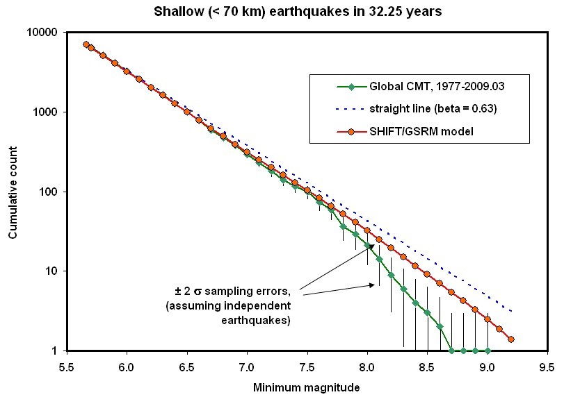
Figure 5. Frequency/magnitude curve of the SHIFT/GSRM long-term shallow earthquake forecast, retrospectively compared to the CMT catalog of 1977-2009.03. No single tapered Gutenberg-Richter model is expected to fit this global composite of different tectonic regimes. Therefore a straight-line Gutenberg-Richter model with spectral slope β = 0.63 is shown for comparison. Error bars on CMT earthquake counts are two-sigma sampling errors if and only if the distribution of earthquake counts follows the binomial distribution; actual sampling errors are probably larger due to earthquake clustering.
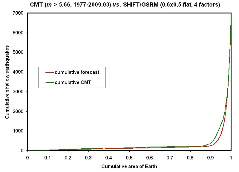
Figure 6. Cumulative
spatial distribution functions for both forecast and actual numbers of shallow
earthquakes above ![]() in a 32.25-year
period. The abscissa is cumulative dimensionless area of Earth surface,
relative to unity for the whole Earth. Grid cells with low forecast
earthquake rates contribute to the left end of each curve, and grid cells with
high forecast rates contribute to the right ends of each curve, as explained in
text.
in a 32.25-year
period. The abscissa is cumulative dimensionless area of Earth surface,
relative to unity for the whole Earth. Grid cells with low forecast
earthquake rates contribute to the left end of each curve, and grid cells with
high forecast rates contribute to the right ends of each curve, as explained in
text.
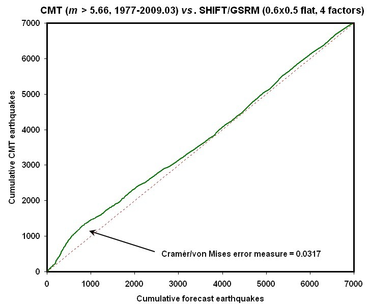
Figure 7. Cumulative
spatial distribution function for actual numbers of shallow earthquakes above ![]() in
a 32.25-year period (vertical axis; ordinate) is plotted against cumulative
spatial distribution function of forecast numbers (horizontal axis;
abscissa). Grid cells with low forecast earthquake rates contribute to
the lower left end of the curve, and grid cells with high forecast rates
contribute to the upper right ends of the curve, as explained in text. An
ideal forecast would yield a straight line with slope of unity, as shown by the
dotted line (except for small variations caused by finite-catalog sampling
errors). See text for discussion of the discrepancy in the lower-left
portion of the curve. The Cramér/von Mises
error measure is the root-mean-square discrepancy between the curve and the
diagonal when both axes are nondimensionalized to range [0, 1].
in
a 32.25-year period (vertical axis; ordinate) is plotted against cumulative
spatial distribution function of forecast numbers (horizontal axis;
abscissa). Grid cells with low forecast earthquake rates contribute to
the lower left end of the curve, and grid cells with high forecast rates
contribute to the upper right ends of the curve, as explained in text. An
ideal forecast would yield a straight line with slope of unity, as shown by the
dotted line (except for small variations caused by finite-catalog sampling
errors). See text for discussion of the discrepancy in the lower-left
portion of the curve. The Cramér/von Mises
error measure is the root-mean-square discrepancy between the curve and the
diagonal when both axes are nondimensionalized to range [0, 1].