![]()
![]()
![]()
![]()
![]()
Step 11: Run statistical-analysis program Slippery
Input file for Slippery:
Preparing your geologic-offsets table (from the previous
step) for input to program Slippery
is very easy:
1. Delete
any row(s) at the top of the table which contain file-header and/or
column-header text(s).
2. File /
Save As / Text (tab-delimited) *.txt.
Perhaps the top of your output file will look something like this (in a plain-ASCII text editor such as NotePad or EditPad Pro):
F0009N
"Arroyo Diablo n.f. W f Bluff M., Quitman Mts.,
TX"
A "Huffington,
1943"
0.4
28.6
C "Stewart,
1978"
<23.7
C "Dickinson,
1979"
15~5 0
A "Stevens and
Stevens,
1985"
<2
B "Hennings et al.,
1989"
3.3
C "Oldow et al.,
1989"
32~27
C "Keller et al.,
1990"
10 3
C "Christiansen and
Yeats,
1992"
28~23 17
C "Frankel et al.,
1996 {slip
rate}"
0
C "Stewart,
1998"
<32
C "Haller et al.,
2002
(904)"
0
F0013N
"normal fault W of Cimarron Mts.,
NM"
A "Smith and Ray,
1943"
2
<66.4
C "Dickinson,
1979"
15~5 0
C "Eaton,
1982"
<17
B "Ingersoll et al.,
1990"
21~15
F0019N
"Teton normal fault,
WY"
B "Horberg et al.,
1949"
<23.7 1.6
B "Love,
1956"
6
~4
B "Love and Reed,
1968"
4.6~6.1
9
C "Stewart,
1978"
<23.7
C "Eaton,
1982"
<17
B "Pierce and
Morgan, 1992"
5
6~4
A "Byrd et al., 1994
(total throw)"
2.5~3.5
0
A "Byrd et al., 1994
(neotectonic rate)"
0.11~0.125
0.075~0.025 0
C "Frankel et al.,
1996"
0
C "Haller et al.,
2002
(768)"
0
C "USGS Q. Fault
& F. D., 2006 (768a, Steamboat Mt.
s.)" 0.0028
~0.015 0
C "USGS Q. Fault
& F. D., 2006 (768b, northern
section)"
.0057~.018
~0.015 0
C "USGS Q. Fault
& F. D., 2006 (768c, central
section)"
.012~.03
~0.015 0
C "USGS Q. Fault
& F. D., 2006 (768d, southern
section)" .014
~0.015 0
C "USGS Q. Fault
& F. D., 2006 (768e, Avalanche Cyn. s.)"
.0052~.007
~0.015 0
F0028N
"Cunningham Park & Big Creek Park n. faults,
WY~CO"
A "De la Montagne,
1953"
0.4
5.3
B "Blackstone,
1975"
5.3
F0034N
"Hoback normal fault,
WY"
B "Love,
1956"
3
~4
B "Armstrong and
Oriel,
1965"
57.8~36.6 0
A "Royse et al.,
1975"
1.8
<57.8
B "Dorr et al.,
1977"
11.2 3.4
B "Corbett,
1982"
11.2
A "Hunter,
1988"
<23.7 >1.6
C "Frankel et al.,
1996"
0
C "Haller et al.,
2002
(772)"
0
C "USGS Quaternary
Fault & Fold D., 2006 (772)"
0.01
0.14 0
F0036R
"Agua Blanca dextral fault,
B.C."
A "Allen et al.,
1960"
11~23
<135
F0360N
"Continental normal fault, WY"
B "Berg,
1961"
0.32
B "Hurrich,
1981"
0.3
23.7 5.3
A "Steidtmann et
al.,
1983"
<5.3
A "Groll and
Steidtmann,
1985"
<~22
A "Steidtmann et
al.,
1986"
<23.7
B "Steidtmann,
1990"
13
A "Steidtmann and
Middleton, 1991"
>13.5
Note that:
(a) There are invisible “Tab” characters separating the fields. These may
display differently in your particular plain-ASCII text editor.
(b) The fault-trace-name field is enclosed in quotations, because these entries
always contain internal blanks. You do NOT want quotation marks around
any of your other fields, so do NOT include any blanks in them.
Prior Distributions of Offset-Rate (for each offset type: D, L, N, P, R, T).
An important decision to make, before running Slippery, is how to provide the Bayesian
“prior” distributions of offset-rate for each class of offset?
Program Slippery uses these distributions to describe (to NeoKinema)
the (very uncertain!) offset-rates of faults that lack dated offset
features.
It also uses these distributions in other (more subtle and pervasive) ways
described in the algorithms of Bird [2007].
An example of one possible prior distribution is shown below: This is for Normal (“N”-type) offset-rates in the western United States [from Bird, 2007]:
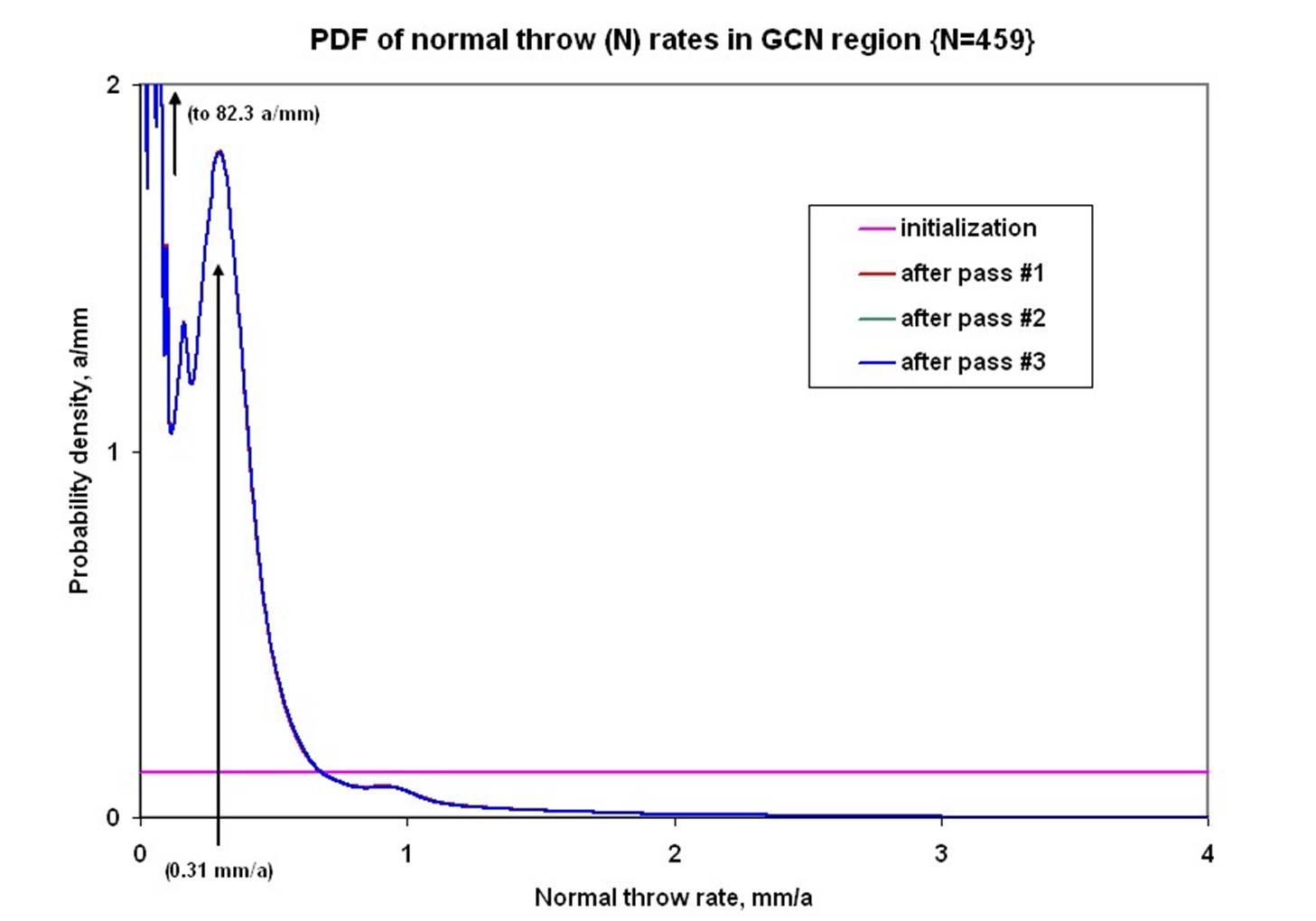
The blue curve here is the Probability Density Function (PDF) of N-type
offset rates. Its units are the inverse of offset-rates, so a/mm (not
mm/a).
A related concept is the Cumulative Distribution Function (CDF) for the same
thing, with is just the integral of the PDF.
Any CDF increases from 0 to 1, and this particular one would give the
probability that an unconstrained N-type offset rate is less than a
certain value.
A complete description of the prior offset-rate distributions contains 6
PDFs; one for each offset type: D, L, N, P, R, T.
The format is one that is intended to be easily loaded into a spreadsheet for
display. The 3 columns are: {offset-rate at bin center, mm/a}, {PDF value
in bin, a/mm}, {offset-rate at right side of bin, mm/a}.
An example is my posted file PDFs_for_L_in_GCN_orogen.txt
Program Slippery can (optionally) read such a file (early in the
run), and it always writes such a file (at the end of the run).
The latter (and later) version is labelled internally as giving “posterior”
distributions, because they have been modified based on the offset-rate data
you provided in your table.
However, the “posterior” distributions from one run of Slippery can
easily be used as the “prior” distributions for the next run of Slippery!
This is an iterative, “bootstrap” method that quickly approaches
self-consistency (meaning that the output is very much like the input).
You have 3 basic options for handling this issue:
(1) If your geologic-offset
database table is large, and it contains representative samples of each of the
6 types of faults with dated offset features,
then you can follow the procedure of Bird [2007]: Do not provide any prior
distributions for the first run of Slippery, but just use the built-in
default distributions.
Then, use the distributions output from this run as the prior distributions for
your second run of Slippery.
Finally, use the distributions output from that run as the prior distributions
for the third run of Slippery.
(2) If your study region has relative plate velocities that are roughly similar to those in/offshore western North America, you might choose to use my posted file PDFs_for_L_in_GCN_orogen.txt as your prior in the first (and only) run of Slippery.
(3) You could load my posted file
into a spreadsheet, and scale each PDF by a constant to decrease (or increase)
the regional activity rates, consistent with lower (or higher) relative plate
velocities.
For example, to decrease all fault offset rates by a factor of 3, you would divide
all offset-rate values (along the x-axis, or abcissa) by 3.
At the same time, you would multiply all PDF values (along the y-axis,
or ordinate) by 3.
In this way, you should obtain a new PDF whose integral is unity. (But,
best to check that numerically in your spreadsheet!)
Actually running Slippery:
When you (finally!) get to run program Slippery, you will have
choices about how many of the intermediate graphs (of various PDFs and CDFs)
you wish to see along the way?
You can turn on all these graphical displays for a more informative
experience.
Or, you can turn them all off to get to the results more quickly.
(This might be appropriate if you run Slippery multiple times.)
If you are watching the graphs individually (and reading the tiny text
messages in the upper-left of your screen), then you will notice:
(a) If Slippery has asked you a question (in tiny text, in the upper-left of
your screen), you should type an answer. Otherwise, the way to move
forward is to press the “Enter” key. (There is no “Back” button!)
(b) Slippery only computes an offset-rate PDF for a table row that has
offset distance and offset age in the same row. Other kinds
of entries, with missing data, generate (non-fatal) error messages, and are
then ignored.
(c) If you entered a positive age in the Before(Ma) column, then offset
finished long ago, and the appropriate offset for neotectonics is
approximately zero. Program Slippery considers this to be a
(mostly) dead fault beneath an overlap assemblage!
Publishable output from Slippery:
One of the output files from Slippery is a table (in tab-delimited .txt
format) that contains both your original input data, and also the new
conclusions from the statistical analysis.
This is intended to be imported into a spreadsheet program, like Microsoft Excel,
or Apache OpenOffice Calc.
Then, adjust the column-widths manually to make it more readable.
Be sure to save this new, expanded spreadsheet (in the
spreadsheet-program’s native format, such as .docx for Excel) for
possible later publication (perhaps as an electronic-appendix, or
supplemental-file).
Remember that if/when you attempt to publish this table, the journal editors
will probably ask you to provide long-form citations for all the source
papers that you cited in your table!
If you kept a stack of photocopies of (at least the first page of) each paper
you cited, then you can build a References Cited manually from your stack of
photocopies.
However, I prefer a different way:
When I discover a useful scientific paper (or book chapter, Open-File Report,
etc.) I immediately enter it into my bibliographic-database
program. (I use Library Master, but there are many choices).
The default record format that I designed has a box for the short-form citation
(e.g., “Love and Reed, 1968”) and also boxes for all the usual long-form
components (first author, coauthors, year, title, journal, volume, pages, DOI,
…, Notes, …).
When I am ready, I can order Library Master to build a long-form
References Cited from any text document that contains the relevant short-form
citations.
And, I can easily produce this text document by taking an extra copy of my
geologic-offsets table, deleting all rows and columns except those containing
the short-form citations, and then exporting as Text (*.txt).
In this way, I was able to produce the file references_cited_in_Table_1.doc, which
accompanied Bird [2007], in only about an hour.
Reformatting output for use in NeoKinema:
Make an extra copy of the Slippery-results spreadsheet
(described in the section above), and save it under another name.
We will now begin to modify its contents and format to gradually turn it into a
fault-offset-rate ASCII table file (f*.nki) intended to be read by NeoKinema.
(However, for convenience we will keep it in the spreadsheet-program’s native
format, such as .docx for Excel, for now.)
First, get rid of all the primary data, and only keep the conclusions:
1. Highlight MOST of the rows in the spreadsheet, except the first
row with the column-headers.
2. Sort all the highlighted rows by: Data / Sort / Column D (“Grade”) / OK.
3. Highlight all rows in which Column D contains “A” or “B” or “C”, right-click
in the highlighted row-number area, and Delete them!
Delete unwanted columns:
1. Note that Column D (“Grade”) is now uniformly filled with “S” and thus is no
longer useful. Delete this column.
2. Delete the new Column D (labelled “Reference”), even though it is not empty.
3. Notice that Columns D, E, F, G are now empty of data. Delete them.
4. Delete the column labelled “mean L” (which should now be column G).
5. Delete the column labelled “mode of L” (which should now be column E).
Re-order the remaining columns:
1. Copy all the lower-limit values from Column D (labelled “l:P(L<l)=2.5%”) and Paste
them in Column K. (Note: This skips over 3 empty columns: H, I, J.)
2. Delete the original of the column you just copied (Column D).
3. Copy all the upper-limit values from Column E (labelled “l:P(L<l)=97.5%”) and Paste
them in Column K.
4. Delete the original of the column you just copied (Column E).
Prepare columns for additional fault-specific data:
1. Label cell F1 with “C?”.
2. Label cell G1 with “ULxKm”.
3. Label cell H1 with “LLxKm”.
Save this reformatted table (still using the spreadsheet-program’s
native format, such as .docx for Excel).
It will be completed in the following steps of this Guide.
![]()
![]()
![]()
![]()
![]()