Step 10: Compile heaves/throws and ages of features offset by each fault train

Before any fault train (or section) can be included in a NeoKinema model (which will estimate its long-term offset rate(s)), 3 conditions must be met:

(A) Fault trace is digitized, labelled, and contained in the f*.dig file.

(B) Constraints on fault offset rate (from analysis of all offset geologic features) are tabulated in an f*.nki file.

Requirement (A) has already been met, in Steps 1 ~ 9 of this Guide.
Requirement (B) will now be considered, in Steps 10 ~ 15 of this Guide.
Requirement (C) will be covered later, in Steps 20 ~ 26 of this Guide.

The best (and easiest) way to fulfill requirement (B) is to perform an automated statistical analysis of all offset geologic features and their ages with my program Slippery, as described in Bird [2007].
This step of the Guide describes how to prepare the input table for that program, by filling-in cells of a spreadsheet with offset distances and their ages from the geologic literature.

I strongly suggest that you build this table in a spreadsheet program, such as Microsoft Excel or Apache OpenOffice Calc.
I will assume use of Excel in these notes.
However, since the spreadsheet will not actually perform any calculations, only the large-table, sorting, formatting, and exporting features of the spreadsheet will be used.

The first task is to prepare a table (in the spreadsheet program) whose first 4 columns are:
            Fnnnn = unique label for the fault trace (train, or section) (5 bytes wide; letter “F” followed 4 digits)
            V = {R, L, N, T, D, P, S} = code for dominant sense of offset (1 byte wide)
            W = {R, L, N, T, D, P, S} = code for secondary sense of offset [or, blank] (1 byte wide)
            Fault trace name = ASCII character string of your choice, possibly containing abbreviations (50 bytes wide)

Fortunately, this will NOT require re-typing all the fault names!
You can import the necessary information from your fault-traces (f*.dig) file in the following way:
            1. From inside Excel, File / Open / Browse / All Files (*.*) / {select your own f*.dig file} / Open.
            2. Select the “Fixed Width” (not “Delimited”) method for defining columns in the input file.
            3. You want to “Start input at row: 1” and Un-check “My data has headers”. Click “Next”.
            4. Click in the sample data window to create column-breaks as listed above: 5 bytes wide, then 1 byte, then 1 byte. Click “Next”. Click “Finish”.
            5. In the spreadsheet, right-click the header for column D and then set Column Width: 50.
            6. Select columns A~H, and then right-click in that highlighted area and: Format / Cells / Number{tab} / Text.
            7. Select columns A~H, and then right-click in that highlighted area and: Format / Cells / Font{tab} / Courier New, Bold, size 9 points.
                        (Note: If your spreadsheet does not offer Courier New font, then choose another “monospaced” font that is available;
                                    Wikipedia has a page called “List of monospaced typefaces” which may help you.)
            8. Save As / Excel Workbook (*.xlsx), using any name you like.
            9. Select the whole spreadsheet (all rows) by clicking on any cell, and then pressing Ctrl + A.
            10. Data / Sort / Column A / OK.
            11. Highlight all the rows that contain (lon, lat) pairs {This is most of the table!}, right-click in that highlighted area, and Delete them!
            12. Highlight all the rows that begin with “***”, right-click in this highlighted area, and Delete them!
            13. Highlight all the rows that begin with “dip_degrees”, right-click in this highlighted area, and Delete them!
            14. Right-click on the header for Column A, and set Column Width: 5.
            15. Right-click on the header for Column B, and set Column Width: 1.
            16. Right-click on the header for Column C, and set Column Width: 1.
            17. Right-click on the header for Column D, and set Column Width: 50.
            18. File / Save.

The next task is manual, but still does not involve much typing; it is mostly done with mouse-clicks and a few keyboard short-cuts: Ctrl+X {Cut} or Ctrl+C {Copy} and Ctrl+V {Paste}.
You need to find every fault train which has a non-blank Column C (secondary sense of offset), and convert that row to a pair of rows.
In each case, you would:
            1. Right-click on the row number just below, and choose: Insert (to create a new, empty row).
            2. Cut the entry from Column C of the upper row, and Paste it in Column B of the (new) lower row.
            3. Copy the Fnnnn number from Column A of the upper row and Paste it in Column A of the lower row.
            4. Copy the fault-trace-name from Column D of the upper row and Paste it in Column D of the lower row.
            5. Consider whether the two fault-names need to be adjusted? (If a fault-trace-name specifies its sense of offset, then that part of the name should be adjusted to agree with the symbol in Column B.)
When this task is done, your table should have Column C completely empty. Right click on the header for Column C and: Delete it.

Next, we need to create a new left-hand column that combines the present Columns A and B.
            1. Right-click on the header for Column A and: Insert (to create a new column A).
            2. Do this again, so that there are two empty columns (now labelled A & B).
            3. Right-click on the headers for the new Columns A & B and set Column Width: 6.
            4. Right-click on the headers for the new Columns A & B and Format / Cells / Font{tab} / Courier New, Bold, size 9 points.
            5. In cell B1, type this formula: “=C1&D1” to concatenate the contents of C1 and D1. Press “Enter”.
            6. Click on the little square at the lower-right corner of cell B1, and drag it all the way to the bottom of the table.
            7. Back at the top of the table, right-click on the header for Column B and: Copy.
            8. Right-click on the header for Column A and: Paste Special / Values / OK. {You do NOT want to copy the formulas, just their results, as 6 bytes of text.}
            9. Delete Columns B, C, D from the spreadsheet.
            10. Insert a new row at the top.
            11. Put column labels in some of these new cells, as follows:
                        cell C1: “Offset(km)”
                        cell D1: “Sigma(km)”
                        cell E1: “Began(Ma)”
                        cell F1: “Ended(Ma)”
            12. File / Save (your spreadsheet).

NOW FOLLOWS THE MOST TIME-CONSUMING STEP IN THE ENTIRE PROJECT:
Find offset features (with known ages) for these faults in the geologic literature, and enter these offsets and ages into the table!

Generically, the procedure is as follows:
            1. Find the right fault in the table. Use: Ctrl + F; {type unique part of fault name}; Find Next; Close. [Caution: This will NOT work right if you have multiple cells selected!]
            2. Right-click on the row number just below, and choose: Insert (to create a new row).
            3. In Column A of the new row, type “A” or “B” or “C” to describe the class of your source, according to the following system:
                        A         original report of new geologic offset from the field, or date from laboratory
                        B         synthesis of geologic data on one basin, range, or other structure
                        C         regional synthesis of geologic data in a state or larger area
            4. In Column B of the new row, type the short-form citation of your source paper. (If you use bibliographic software like Library Master to keep track of these, try to match the short-citation text exactly.)
            5. In Column C of the new row, type the offset distance in kilometers. Use “~” to separate two numbers defining a range. Use “>” as a prefix to a lower limit. Use “<” as a prefix to an upper limit.
            6. If your source gives the standard deviation (standard error) for the offset, type this in Column D of the new row. Otherwise, leave it blank.
            7. In Column E of the new row, type the age of the offset feature in Ma. Use “~” to separate two numbers defining a range. Use “>” as a prefix to a lower limit. Use “<” as a prefix to an upper limit.
            8. If the fault continues to be active, insert “0” (zero) in Column F of the new row. [Otherwise, do you really want to include this fault in a neotectonic model?]

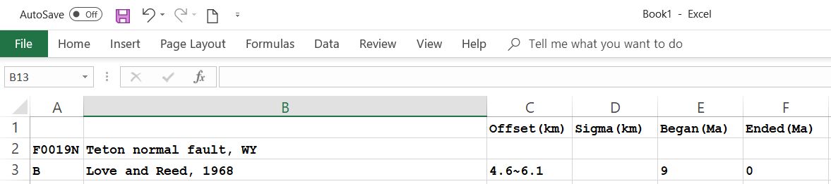
To give a specific example, suppose that you read about the Teton normal fault of Wyoming in the following book:

John David Love and J. C. Reed, Jr. [1968] Creation of the Teton Landscape: The Geologic Story of Grand Teton National Park, Grand Teton Natural History Association, Moose, WY.

and you captured these essential facts: That the Teton normal fault began to slip at 9 Ma, and that the total throw (relative vertical displacement) since then has been 4.6 to 6.1 km. The fault is still active.
You would enter this information in the spreadsheet as follows:

It is possible that you will find estimates for dip-slip offsets that include both throws (type “N” or “T”) and heaves (type “D” or “P”).
Note that you may not mix throw and heave rates for a single fault trace; you have to choose one option or the other.
(But, it would be easy for you to convert a throw to a heave. or vice versa, on a calculator--if you know the fault dip.)
Be sure that character#6 in the fault-trace-number in Column A agrees with your final choice of offset type.
(But, it is not critical that this character should agree with the dominant-offset-type character originally listed in your f*.dig file. Those are only used to select line-colors when plotting traces.)

Note that you can (and should) include as many offset features as you can find for each fault train or section.
Even small (Holocene?) offsets of a few meters are useful if their ages can be constrained. [Remember: 1 m = 0.001 km; and 1 ka = 0.001 Ma. Enter in the table using units of km and Ma.]
Do not be too concerned if the different offset-rates do not seem to agree; program Slippery will reconcile them (in the next step).

Also, do not be overly concerned if some of your faults have NO offset features. This is common.
(Programs Slippery and NeoKinema can deal with such cases; they use different, powerful methods.)
Just leave all such “unconstrained” fault trains in your table, so that program Slippery will provide broad offset-rate ranges (in the next step).

BE ALERT FOR ANY EXISTING COMPILATIONS OF GEOLOGIC DATA THAT YOU CAN MINE!
If your model region includes the western United States, consider data in both Tables 1 & 2 of Bird, 2007, and also from Table 4 of Bird, 2009.
You will not be able to automate the import process (because fault-trace-names may differ, and Fnnnn numbers will definitely differ!),
but transferring numbers and citations from one table to another is MUCH quicker than finding and reading papers, either in the library or on-line.

What if you come across a paper that gives a geodesy-based estimate of neotectonic offset rate?
Usually, my preference would be to leave those out of this “geologic” table, but to include these geodetic-velocity data in the geodetic dataset that we will build in Steps 16~19 of this process.
However, if it is impossible or impractical to obtain that geodetic data (or if its velocity reference frame is unclear or non-standard) it may be best to include that rate estimate here.
In that case, remember that you cannot enter a rate directly; you would have to express it as an offset since some age.
For example, “4~6 mm/a” might be entered as offset of “0.0004~0.0006” km since “0.0001” Ma (that is, 0.4~0.6 m since 100 years ago).
Also, be sure that you convert total slip-rate to some dominant component of offset-rate; these are only the same for pure “R” and pure “L” faults.