Step 31: Plot interpolated stress directions with NeoKineMap

It is important to make visual checks to ensure that stress-directions have been imported without error,
and also that the interpolation of stress-directions within NeoKinema was reasonably successful.

NeoKineMap makes it easy to plot both of these datasets.
You can probably re-use your previous choices of (virtual?) paper-size and map-projection, unchanged.
When NeoKineMap asks, “Do you want one (or more) of these mosaics?”, answer “No.”

For the first map, I suggest that you combine two Overlays:
  1 :: digitized basemap (lines type)
            which will be your basemap .dig file with coastlines, statelines, etc.; AND
12 :: stress direction data
            which will be your s*.nki input data-file.

For the second map, I would suggest that you combine three Overlays:
  1 :: digitized basemap (lines type)
            which will be your basemap .dig file with coastlines, statelines, etc.; AND
  2 :: outline of F-E grid
            which will be based on your active .feg file, AND
13 :: stress directions interpolated by NeoKinema
            which will be your new s*.nko output-file.
            NOTE that there may be many thousands of interpolated stress-directions
            (if your .feg file has thousands of elements).  Fortunately, NeoKineMap
            will offer an option to plot only a fraction (1 / N) of these.  Try N = 9?

The following pair of (successful) plots is from Bird [2009]:

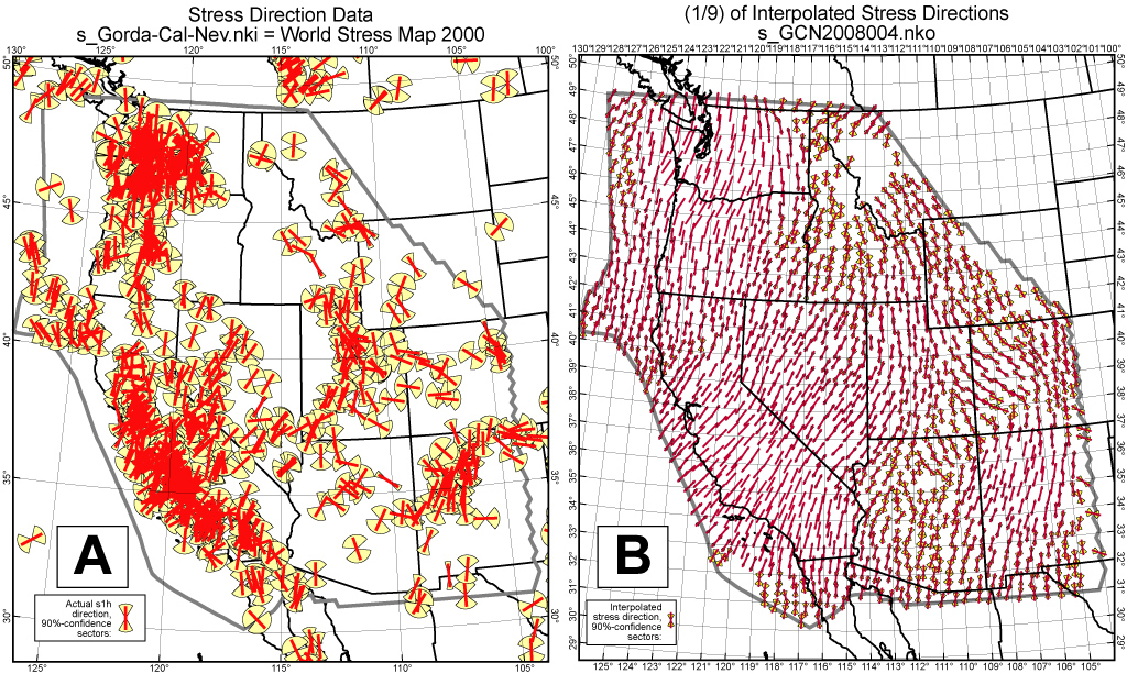
If your input data (in the left plot) are not as numerous as in my example, or if they are very noisy (i.e., internally inconsistent),
then one possible problem might be that your interpolated stress directions (in the right plot) have too many “white holes”
where no stress-direction could be inferred. 
In that case, you can go into your NeoKinema-parameter file p*.nki, and change the logical value in line #11:
            FALSE           switch: Do active faults give sigma_1h direction data?
If you change this to TRUE, then NeoKinema will infer a stress-direction from the rake (offset-sense) of each
active fault included in your model.  These “pseudo-data” may help you to get a more reasonable interpolated map
(after re-running NeoKinema, and re-plotting with NeoKineMap).

The paragraph above may cause you to wonder:  Why is inference of stress-direction from active faults not the normal, default choice?
It is because the relationships between fault traces and stress-directions can be complex.
There are at least two reasons that we are beginning to understand:

· Dynamic F-E modeling (i.e., with Shells) has shown that most active faults have much lower coefficients of (effective) friction
than the unfaulted continuum (microplates) between the faults.
This contrast in lithospheric strength requires certain stress components to change around faults,
which causes principal stress directions to locally rotate around faults.

· Many faults active in the Holocene were created in earlier geologic times (e.g., Cretaceous, Paleogene, …)
when stress-directions were probably different from today.
However, the fault trace is fixed in the bedrock, and not free to rotate as stress-direction changes
through geologic time.  (Therefore, some old faults may have reversed their slip-senses during long histories.)

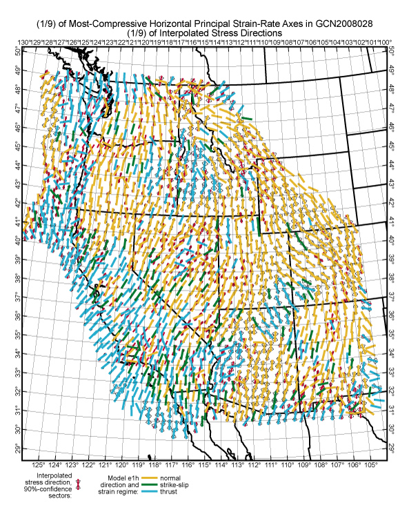
One more suggestion, while we are on the subject of stress-direction maps:
The interpolated stress-directions in the right plot above are the targets for the orientations of principal axes of strain-rate
in unfaulted (continuum) elements in your NeoKinema model.
However, for various reasons the resulting calculated principal strain-rate axes may differ.
It is easy to obtain a map which shows exactly where the misfits are, and how large they are:

You can probably re-use your previous choices of (virtual?) paper-size and map-projection, unchanged.
When NeoKineMap asks, “Do you want one (or more) of these mosaics?”, answer “No.”

For this comparison map, I suggest that you combine three Overlays:
  1 :: digitized basemap (lines type)
            which will be your basemap .dig file with coastlines, statelines, etc.; AND
13 :: stress directions interpolated by NeoKinema
            which will be your s*.nki input data-file.
11 :: most-compressive horizontal principal strain-rate axes.

If you plot the overlays in this order, then successful principal strain-rate directions
(plotted in blue, yellow, and green, depending on neotectonic strain-rate regime)
will overlay and hide the interpolated stress directions (plotted in red).
You will only be able to see the cases with a significant angular misfit.