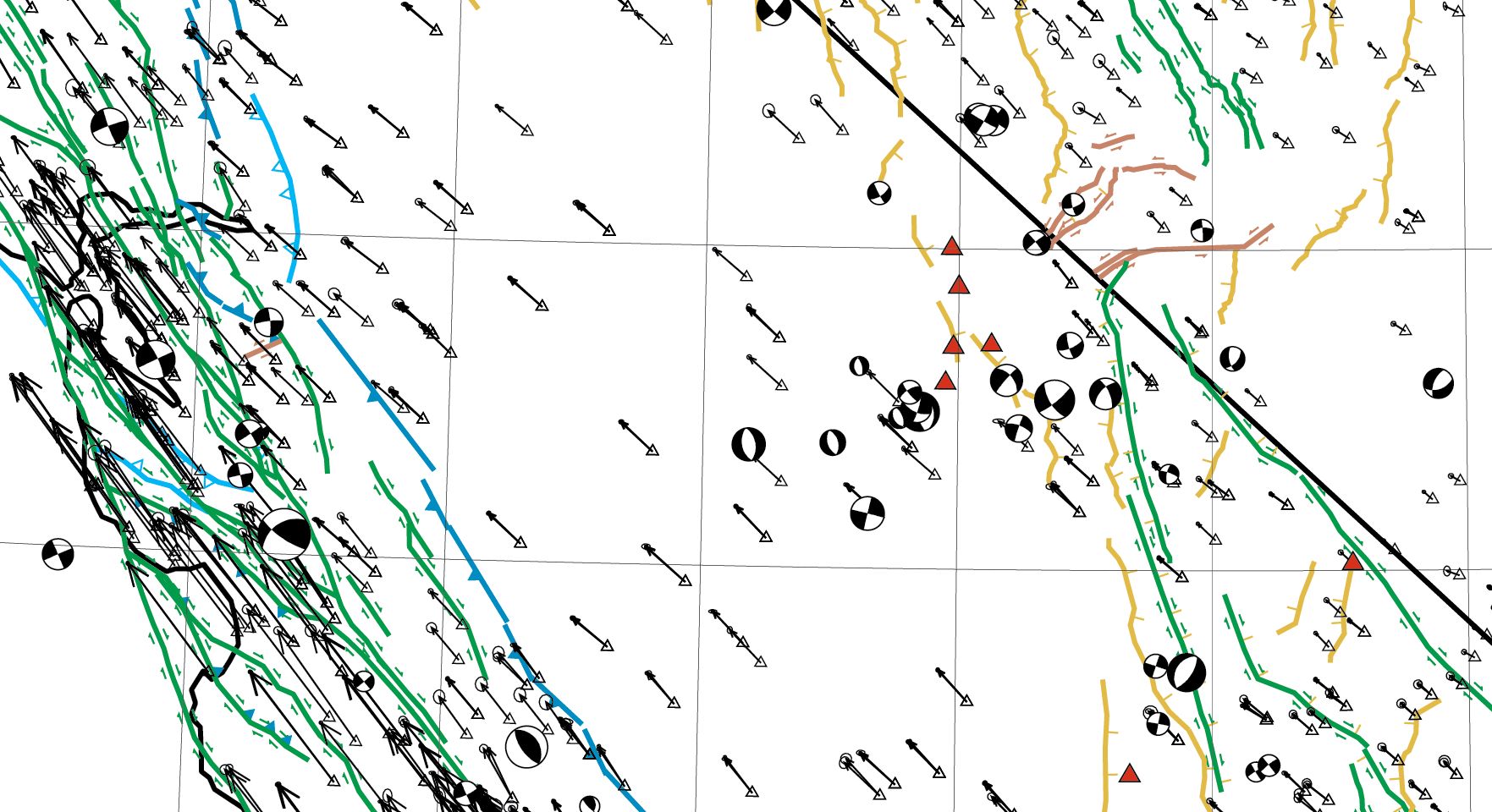
Step 18: Plot GPS velocities and look for noise processes(?)

In this step we will make a map of steady(?) interseismic(?) GPS velocities of benchmarks from your .gps file, and their spatial relations to various potential noise sources.

Plotting NeoKinema-related maps with program NeoKineMap was already introduced in Step #8.
You can choose any name for this new map plot, as long as it ends in characters “.ai”.
If you have already made a plot with this program, it should remember your previous choices about (virtual) paper size, map projection, map center, and map scale; these are recorded in its Map_Tools.ini file.
Whether or not you used a very large “virtual” page for your last map, that would be a good choice now, because the suggested new map consists of 5 kinds of overlays:

When NeoKineMap offers to plot a (colored-area) “Mosaic” layer, decline this offer, with “No”.

When NeoKineMap offers a choice of (line-based) “Overlay” layers, begin with:
1 :: digitized basemap (lines-type)
because this gives you the chance to plot your file of coastlines/state-lines/border-lines, in (longitude, latitude) coordinates, that you created earlier, in Step #4 and Step #5.
If you don’t have such a file, perhaps you could use North_America_states.dig or WorldMap.dig which are posted on my web site.)

When NeoKineMap asks, “Do you want additional overlays?” answer “Yes”.
Then select overlay type of:
4 :: fault traces
and then enter the name of your digitized-fault-traces file, in (longitude, latitude) coordinates, ending with “.dig”.

When NeoKineMap asks, “Do you want additional overlays?” answer “Yes”.
Then select overlay type of:
8 :: geodetic benchmarks with velocities
and then enter the name of your .gps file, just recently finalized in Step #16.
The plot-type index you should select is #1: observed geodetic velocities…
The number of “Ma” (millions of years) that you select (for velocity extrapolation) will determine the size of all the GPS velocity vectors;
generally a good choice is somewhere in the range of 1 ~ 10 Ma.  [ Remember: 1 mm/a = (1 km) / (1 Ma). ]

When NeoKineMap asks, “Do you want additional overlays?” answer “Yes”.
Then select overlay type of:
14 :: earthquake epicenters from …. file
to plot locations of large (m > 5), shallow (z < 70 km) earthquakes.  My web site provides utility program Seismicity to produce an .eqc (EarthQuakeCatalog) file,
which you should place in the active folder where NeoKineMap is reading its other current input files (like .dig and .gps).
Note that a data file is also provided (for Seismicity) which contains a condensed form of the Global Centroid Moment Tensor (GCMT) earthquake catalog.

When NeoKineMap asks, “Do you want additional overlays?” answer “Yes”.
Then select overlay type of:
15 :: volcanoes (Recent, subaerial) from file …
to plot Recent volcano locations.  My web site provides a dataset from the Smithsonian Institution’s Global Volcanism Project [Simkin & Siebert, 1995]
which you should place in the active folder where NeoKineMap is reading its other current input files (like .dig and .gps).

As you finish up the map in NeoKineMap, be sure to include a (longitude, latitude) graticule of parallels and meridians, probably with spacing of 60 minutes (1°).

Open the resulting map plot in Adobe Illustrator.
The resulting plot may be quite busy and crowded!
Note that Adobe Illustrator makes it easy to select groups of objects (with the black-arrow Selection Tool), and then use: Object / Hide / Selection
to temporarily remove annoying information (like fault F1234R numbers, and benchmark names) from the map, without actually deleting them!
Also notice that you can use the Zoom Tool (magnifying glass) to view only a small area of the map.
You can also use the Hand Tool (glove) to easily move the map relative to your viewing window.

If you decide that the plot has to be re-done (for example, to shorten the GPS velocity vectors?),
it will be much faster to create next time, because all your previous choices will be remembered.

What should you look for on this map?
Well, one expects that GPS velocity vectors will show changes across the traces of active faults.
However, do you see any recent earthquake that seems to be associated with other kinds of motions?  Make a note of its location; then look in the .eqc file for its date and other parameters.
Or, if you see a volcanic center which seems to be associated with a radial pattern of (outward or inward) GPS velocities?  Again, make a note of its geographic (longitude, latitude) coordinates.

If you see any areas of anomalous GPS velocity, it is possible that some natural “noise” processes (other than steady interseismic strain accumulation)
are present in your .gps dataset.  Instead of deleting benchmarks and their velocities, we can deal with this, in the next Step, by augmenting (or creating) the .gp2 matrix.