Step 22: Create fault-corridors in your grid?

Unlike F-E grids (.feg files) intended for use with program Shells, F-E grids intended for use with NeoKinema contain NO linear (red-line) fault elements.
Instead, fault traces are supplied directly to NeoKinema through your f*.dig file (which we created earlier, in Guide Steps #1 through #9).
This means that, in principle, you might not need to adjust your F-E grid to reflect the positions of faults.

In my 2009 NeoKinema model of the Gorda-California-Nevada orogen [Bird, 2009] I decided not to refine my F-E grid in the offshore region called the “Gorda plate” (although “Gorda orogen” would be a more appropriate name).  Chaytor et al. [2004] had used high-resolution swath bathymetry and seismic reflection profiling to define 545 active or potentially-active faults in the region, which was an overwhelming number.  Also, there seemed to be little point in trying to model them individually, because (a) only one of these faults had a geologic offset-rate constraint; (b) none of these faults had GPS benchmarks nearby; and (c) no one lives anywhere near those faults, so their seismic hazard does not imply any seismic risk.  Therefore, I just left the auto-generated F-E grid created by command Tools / TileRegionalGrid [in OrbWin] to represent those 545 faults, as shown below.  The result (in the final NeoKinema models) was to make the whole region about equally weak.  Below you can see how this grid looked within OrbWin:

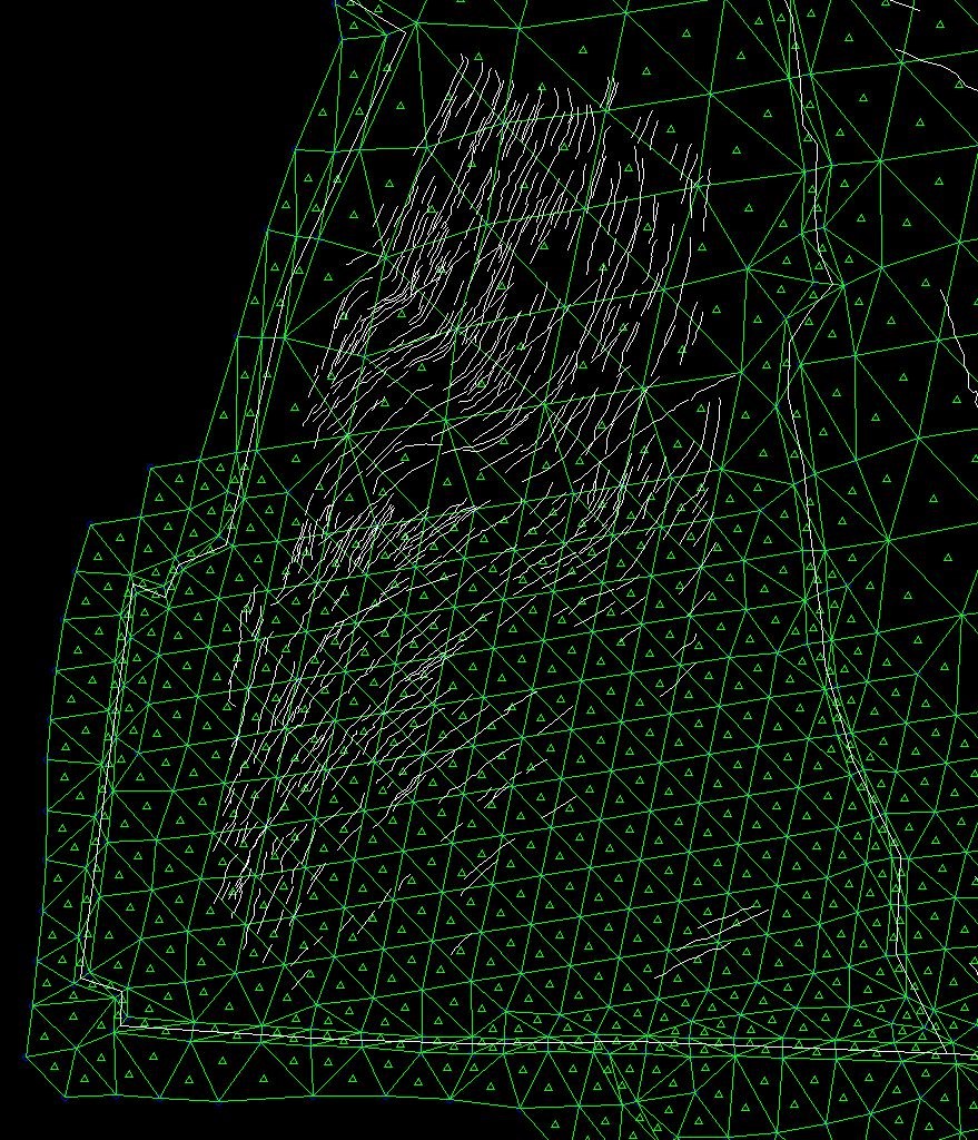
However, as the figure above also shows, I outlined the fast-moving plate-boundary faults
(Mendocino transform fault, Gorda Rise spreading center, and Cascadia Trench) with “fault-corridors” of narrow triangular continuum elements.
Also, I used fault-corridors for all the major (fast-slipping) faults on land in the western United States.
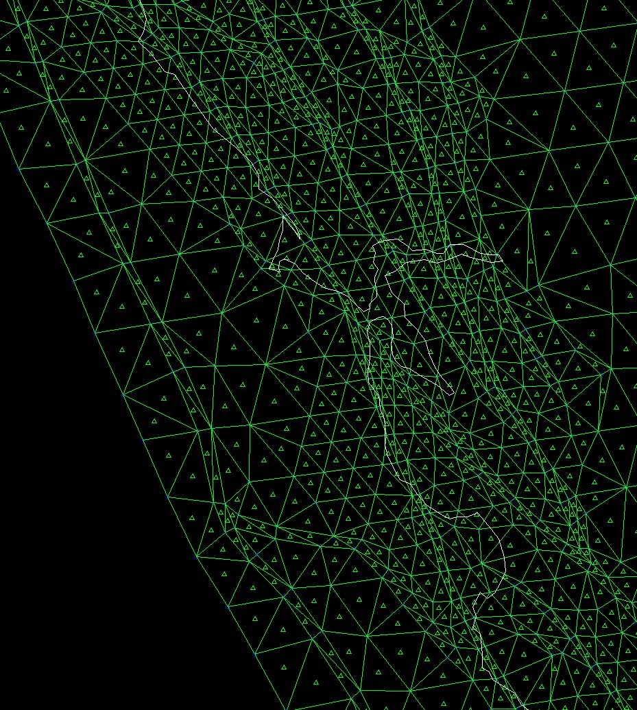
For example, the next image shows a part of the grid from the San Francisco Bay area (with only the coastline shown in white; fault traces omitted for clarity):

There are some major advantages to defining “fault-corridors” in your .feg file (although it is somewhat laborious):

(a) NeoKinema does not actually represent faults with velocity discontinuities; it represents them with zones of enhanced weakness and higher strain-rate.
A narrow zone of enhanced strain-rate is a better approximation of a velocity discontinuity than a broad zone is.

(b) The exact shapes of fault traces, and relationships between fault traces (especially strike-slip fault traces),
create an anisotropy and inhomogeneity in the regional strength that is captured better if you use narrow fault-corridors.

(c) NeoKinema detects all cases of GPS benchmarks within the same triangular finite-element as a fast-slipping faults, and requires you to remove these GPS benchmarks from the input data.
If the fast-slipping faults are confined to narrow fault corridors, then the number of GPS benchmarks removed can be minimized, and the number of GPS data kept in the simulation can be maximized.

Assuming that you decide to define fault-corridors (at least along fast-slipping faults, >1 mm/a, on land), the procedure is fairly simple:

(1*) Use command Edit / Add/Delete Element to delete existing elements and thus clear some space around a group of faults.  Also delete any unconnected nodes. 

(2*) Use command Edit / Add/Drop Node to create pairs of new nodes, spaced periodically along the trace of each fault.  Where a fault ends without connecting to another, place a single new node just ahead of this propagating tip.  Around a triple-junction between 3 faults, place 3 new nodes (one on each microplate).  Around a quadruple-junction, place 4 new nodes, et cetera.

*As of January 2018, a new utility program called Fault_Corridors is available to automate steps (1) and (2) above.  It reads an .feg file without fault-corridors, and a f*.dig file with digitized fault traces, and uses these to create a new .feg file with fault-corridors.  It is still a bit buggy(!)  Also, it will still be necessary to manually perform steps (3), (4), and (5) [described below], back inside OrbWin again.

(3) Finally, “sew” together the new nodes and the existing nodes by using command Edit / Add/Delete Element to create new elements, filling any holes in the lithosphere.

(4) Check that the fault-corridors actually enclose all of the fault traces, and use command Edit / AdjustNode as needed.

(5) Use the topological test: Tools / Perimeter/Area Tests and then the visual test: Tools / View Gaps/Overlaps to detect any remaining problems with your new grid.
Fix any problems immediately, before moving on to edit a new area.
When done, use command File / SaveGrid.