Step 33: Run NeoKinema many times with different weights

At the end of each run of NeoKinema, a summary table of misfit measures (for each data class) is produced.
On your monitor screen, and also at the bottom of the log-file t*.nko, you will find something like this:

================================================================
Continuum    errors: N0 = 0.055, N1 =     0.526, N2 =     1.366
Stress       errors: N0 = 0.115, N1 =     0.876, N2 =     1.831
Offset-rate errors: N0 = 0.016, N1 =     0.198, N2 =     0.618
Potency-rate errors: N0 = 0.094, N1 =     0.806, N2 =     1.612
Geodetic     errors: N0 = 0.374, N1 =     1.954, N2 =     2.699
================================================================

The greatest possible number of rows in this table is 5 (Continuum, Stress, Offset-rate, Potency-rate, Geodetic).
If you are running a model with no stress-direction dataset, or with no GPS-velocity dataset, fewer lines will appear.
The explanation of the row-names is similar to that in the previous Step, but with one addition [“Potency-rate”]:

§ Continuum (i.e., long-term-average {non-elastic; permanent} strain-rates different from zero in unfaulted elements)

§ Stress (i.e., azimuths of most-compressive principal strain-rate different from interpolated stress directions; see last Step)

§ Offset-rate (i.e., differences between geologic target offset-rates of faults, and model rates)

§ Potency-rate (similar to Offset-rate misfits, but re-weighted to emphasize large, fast faults with high seismic hazard)

§ Geodetic (i.e., long-term-average benchmark velocities different from GPS rates {after correction for model seismicity rates})

As explained in the previous Step, each single misfit is made dimensionless by dividing by its assigned datum uncertainty σ,
and each misfit is also converted to a positive dimensionless number (of O(1)) by taking its absolute-value.
So, within each data-class, we have a long list of positive, dimensionless misfits, of O(1). How to summarize them?
NeoKinema uses 3 different well-known metrics (N_i, short for “norms”) to describe these strings of numbers:

Ø N₀ is the fraction of dimensionless misfits that exceed 2.0. [Ideally, it should be ~0.05.]

Ø N₁ is the mean absolute value of the dimensionless misfits. [Ideally, it should be ~1.0.]

Ø N₂ is the RMS (root-mean-square) of the dimensionless misfits. [Ideally, it should be ~1.0.]

The N₂ norms are most important, because they are most similar to the terms in the objective function that NeoKinema
was told to minimize. (That is, they represent the most “fair” tests of whether NeoKinema did its job properly.)
In Bird [2009], paragraphs [17~18] and equations (2~4) give specific definitions of these N₂ norms for each class.
The same section also explains why the “Potency-rate” misfit measure is much more useful than “Offset-rate”.
However, I would like to make one small update to the text of that paper. When discussing Geodetic N₂, it says,
“…this error measure at each benchmark involves only the local (2 × 2) covariance of its two horizontal components…”
This is still true if the user provided NO GPS-covariance matrix (.gp2) for that run of NeoKinema.
However, in NeoKinema_v5.2+, the full .gp2 covariance matrix is used to compute Geodetic N₀, N₁, N₂ when available.

Since I have now explained why the N₂ norm is more important than either N₀ or N₁,
and I have also explained why “Potency-rate” is a more useful misfit measure than “Offset-rate”,
let’s look at the same table with the less-important information grayed-out,
and the most important numbers highlighted in yellow:

The goal of this step in the NeoKinema modeling process is to make many runs, with different weighting
factors, and try to get all the “yellow” N₂ values above to lie in the general range of 1 < N₂ < 2.
Values of 1.0 would be ideal, in the “fantasy” case where all data errors are properly described by their σ’s,
and there are no conflicts between classes of data, and no numerical errors or approximations in the code!
Values of less than 1.0 are actually not desirable, because the model is then “overfit” to the data;
this means that even the small random-noise component in the dataset is being fit!
On the other hand, most researchers consider N₂ misfits of >2.0 as showing a model that is “underfit”,
in the sense that it has misfits more than twice as big (on average) as the expected noise level in the data.
In other words, typical model predictions are falling outside the prior “95%-confidence bounds” on the data.

The best way to balance the N₂ norms for the Stress, Potency-rate, and Geodetic data classes is to modify L₀ and A₀:

Ø To reduce the Potency-rate N₂ norm, reduce L₀.

Ø To reduce the Stress N₂ norm, reduce A₀.

Ø To reduce the Geodetic N₂ norm, increase both L₀ and A₀.

An example of such a search in (L₀, A₀) space [at fixed m, ξ ] is given by the following figures from Bird [2009].
First, the “response” of each N₂ norm is shown separately; then, all 4 graphs are overlain:

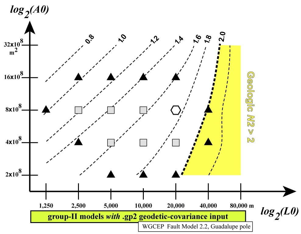
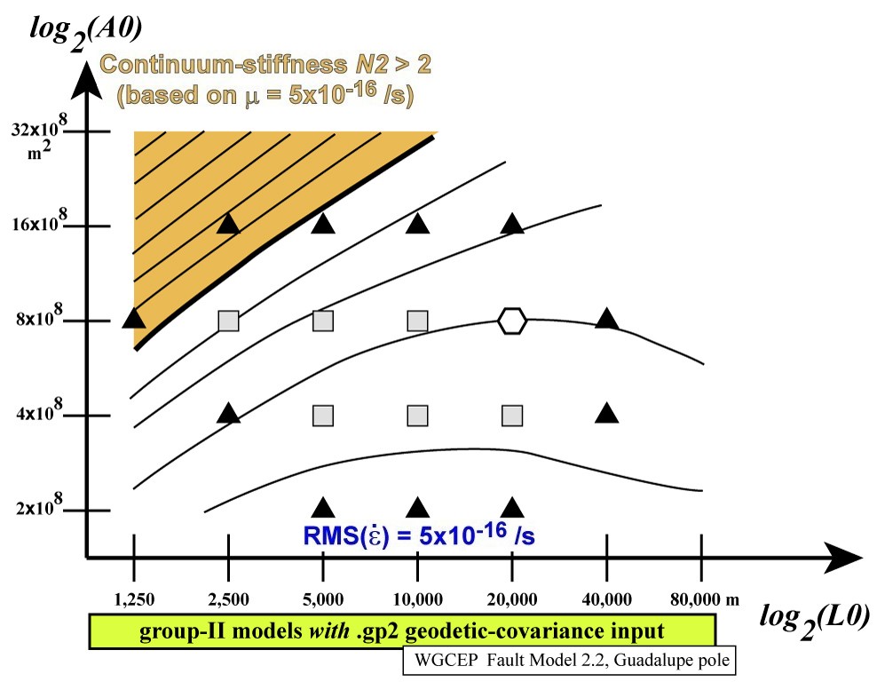
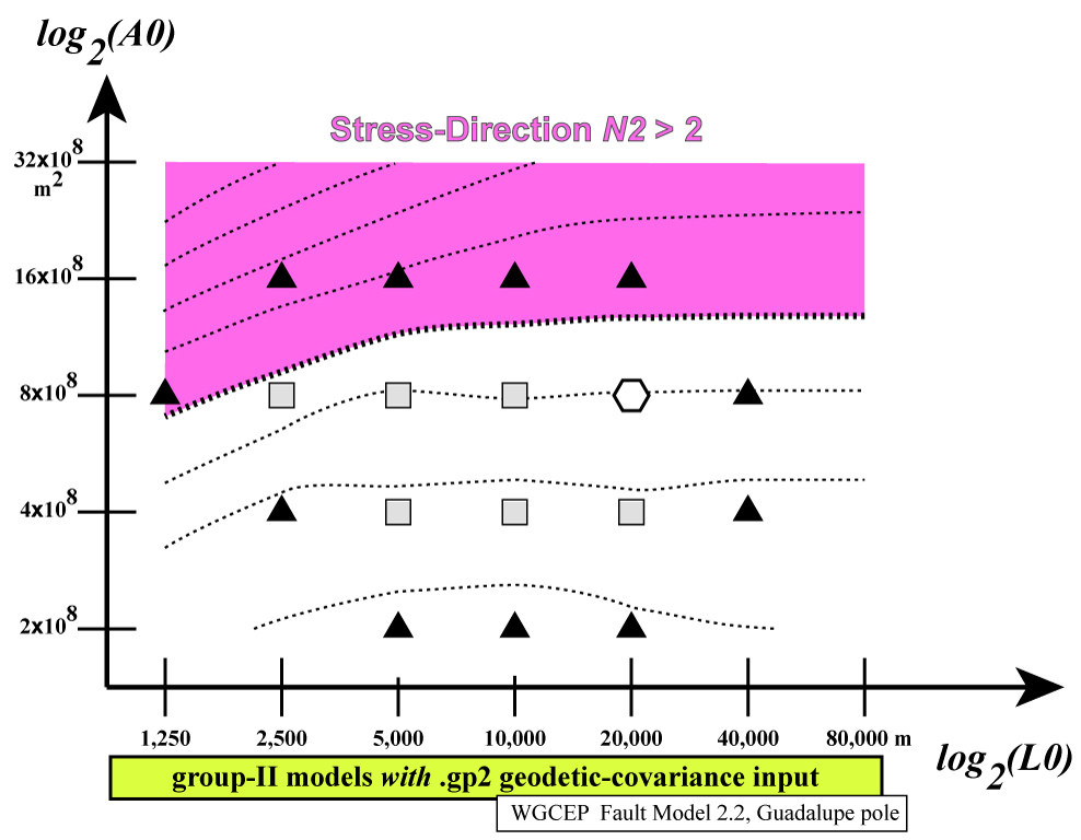
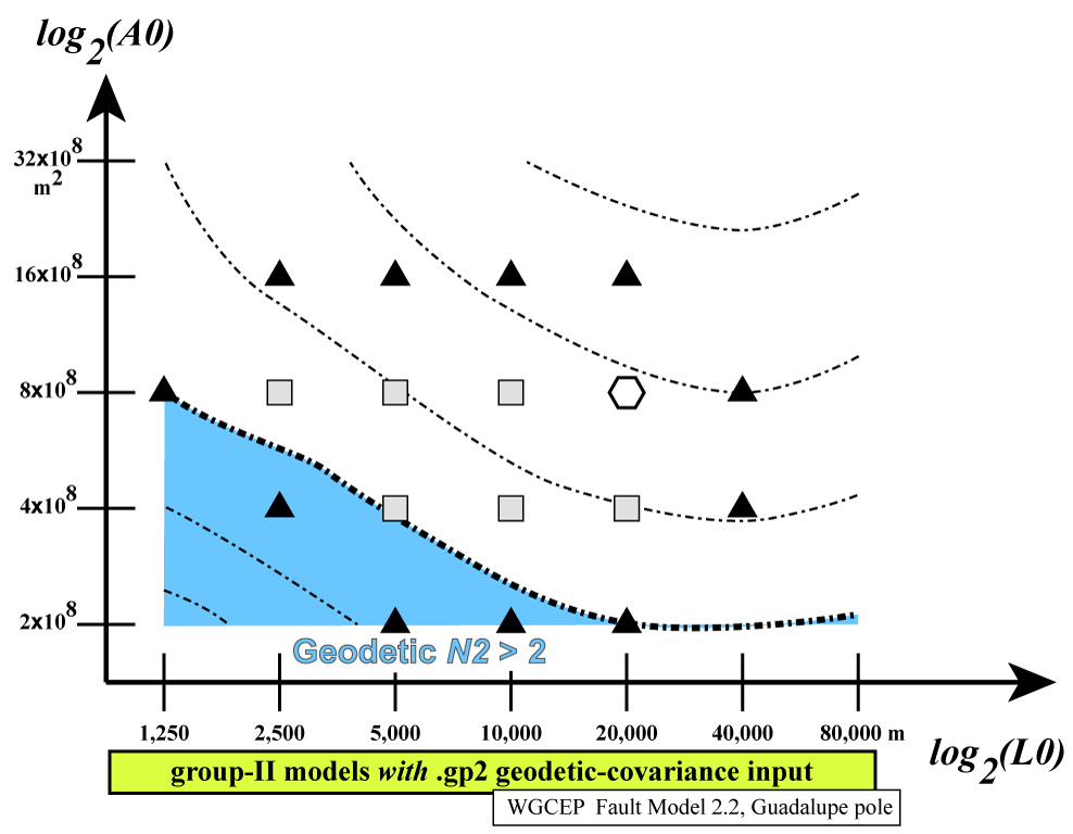
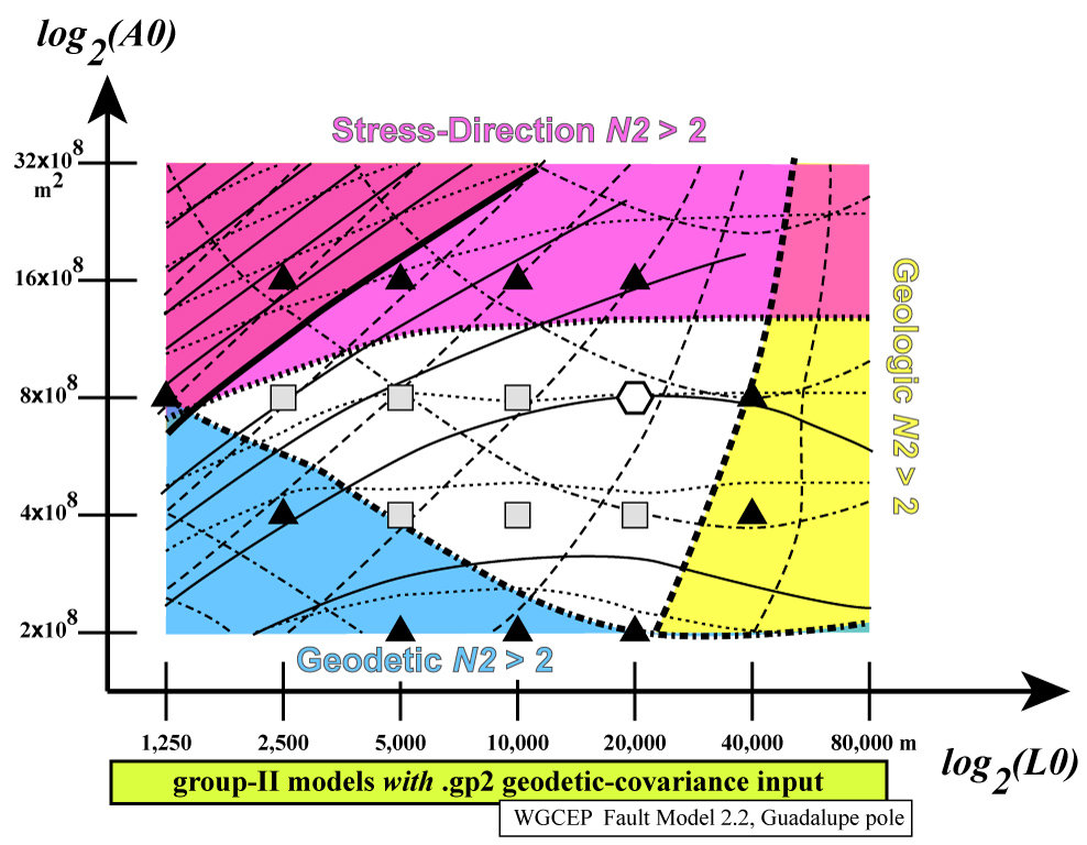
Notice how the colored areas (showing some N₂ > 2) reject all extreme values of (L₀, A₀),
while the central “white space” shows a range of acceptable models.
Among these acceptable models, the preferred model (hexagon) is the one which has roughly equal N₂ values for each data-class.

(If the data in your problem are harder to fit, and there is no white-space, then you could redefine the colored areas as:
N₂ > 2.2, or as N₂ > 2.4, etc.)

The adjustment of weighting parameter m is relatively easy, for three reasons:

1. You can always reduce the Continuum N₂ norm by increasing m, and vice-versa.

2. At the end of each NeoKinema run, the text-output will include both the “Root-Mean-Square” and “Mean (absolute) value” measures
of continuum strain-rate. You can always try a m within this range in your next run, working toward a self-consistent model by a “bootstrap” method.

3. Once “preferred” values of (L₀, A₀) are determined, you can hold these fixed, and experiment with varying only m, as in this figure [Bird, 2009]:

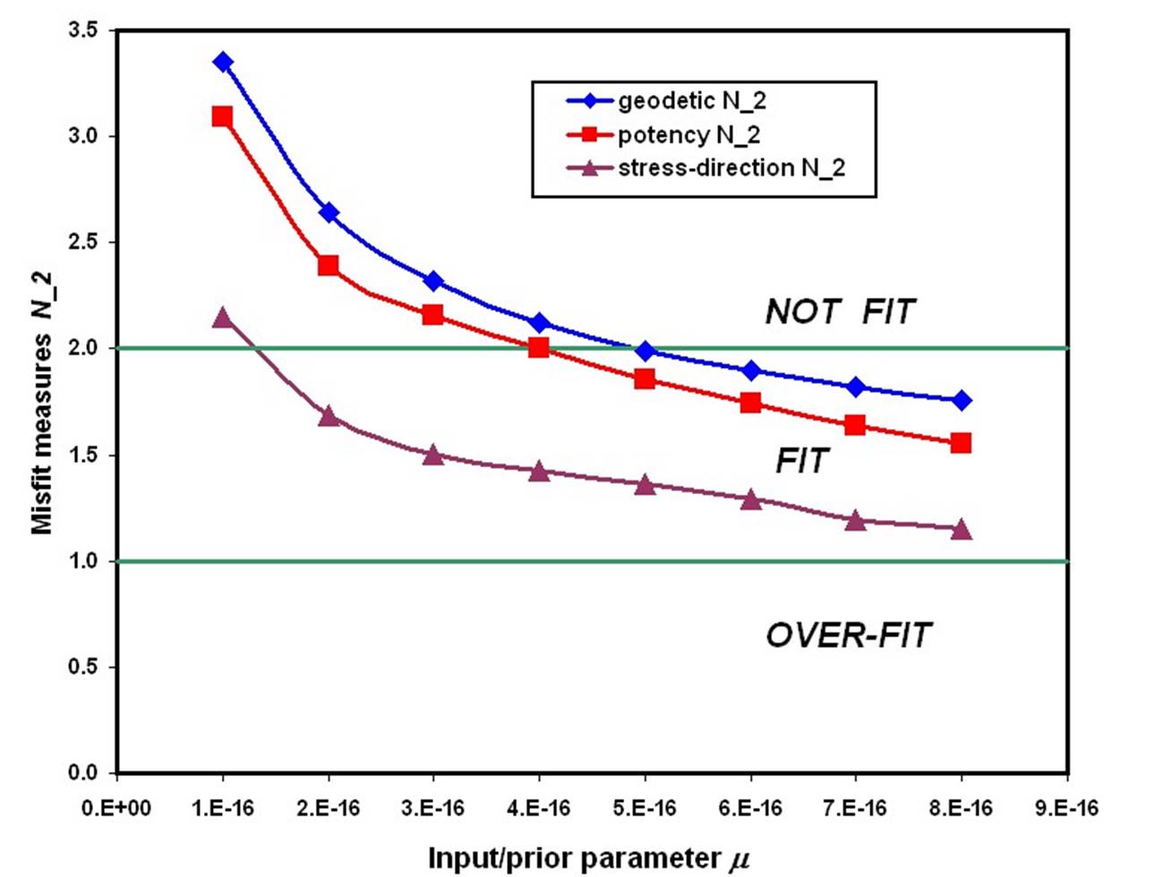
I suspect that you will find there is some minimum value of m, below which the other data-classes can not be adequately fit.

The effects of varying ξ are the most subtle, so I would suggest postponing those experiments for the end of the project.
If you get that far, make “Mosaic” map-plots of type #9 :: “continuum long-term-average strain-rate, excluding modeled faults”
in NeoKineMap to see the effects of varying ξ most directly.