![]()
![]()
![]()
![]()
![]()
Step 34: Tabulate the fault slip-rates in preferred & acceptable models
If you are using NeoKinema as a “deformation model” in a
seismic-hazard-estimation project
[e.g., Field et
al., 2013; Petersen et al., 2014], then one of the key products
will be a set of preferred fault slip rates.
This information is implicit in the NeoKinema input and output files, but dispersed:
Ø Fault dips (needed to
convert throw-rates and heave-rates to slip-rates and rakes) are in the f*.dig
input file
(as dip_degrees tags), or
else built-into NeoKinema as generic default dips.
Ø Fault names (and also the logical markers for aseismic slip) are in the f*.nki input file and the f*.nko output file.
Ø Model predictions of
offset-rate components (throw-rates and heave-rates) are in the f*.nko
output file.
(However, for any oblique-slip fault the strike-slip rate and the dip-slip-related
rate are in separate rows.)
I have written a utility program to bring these together and create a table:
Rake_And_Sliprate_Per_Fault.
This will read the parameter file (p*.nki) that you choose (associated
with your preferred model);
and then use this to identify the f*.dig file that was used in NeoKinema,
and read that;
and also identify the f*.nko file of output that was produced by NeoKinema,
and read that.
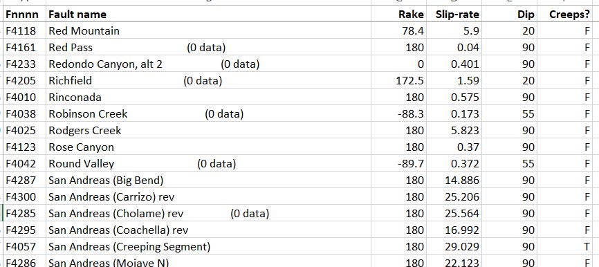
This utility produces a tab-delimited plain-ASCII table file, *_rake_and_sliprate_per_fault.txt,
where * is the model-identifying name-token of your preferred model
(from the first line of your p*.nki).
You should open this output file with a spreadsheet (such as Microsoft Excel,
or Apache OpenOffice Calc)
and format it for display (or output to .pdf, …). It might then look
like this excerpt:
A very common question, at this point, is: “Does
NeoKinema provide uncertainties for predicted fault slip-rates?”
The short answer is: “No. It only provides a
posterior best-estimate of the average slip-rate of each fault, in some preferred
model[s].”
However, we can supply a fuller answer by “unpacking” the two qualifiers in that short answer.
First, let us consider the phrase, “in some
preferred model[s]”.
“Preferred” (or maybe “acceptable”) models usually means “all models whose
worst N2 misfit-norm was still less than 2.0 (or perhaps
a higher cut-off)”.
(This was discussed in the previous Step.)
This class of “presentable models” might include, for example:
Ø Models with a range of (L0, A0) weighting parameters;
Ø Models with varying fault models (e.g., UCERF3 Fault Models FM3.1 versus FM3.2);
Ø Models with slightly different Euler poles for the plates that drive the boundary-conditions (see Step 26).
I have written a different utility program to summarize the range
of offset-rates found in a group of “preferred models”.
RangeFinder reads in a
group (as large as you like) of f*.nko output files, and produces
a tab-delimited, plain-ASCII, flat-file table file (e.g., RangeFinder.txt) that you can
open in any spreadsheet.
The table has columns with the range of offset rates for each fault, and also
other columns that give
the magnitude of the range (so you could sort by magnitude, to find the most-uncertain
rates), and
also columns that identify the two NeoKinema models that had the highest
and lowest offset-rates for that fault.
An excerpt from some RangeFinder output is shown below:
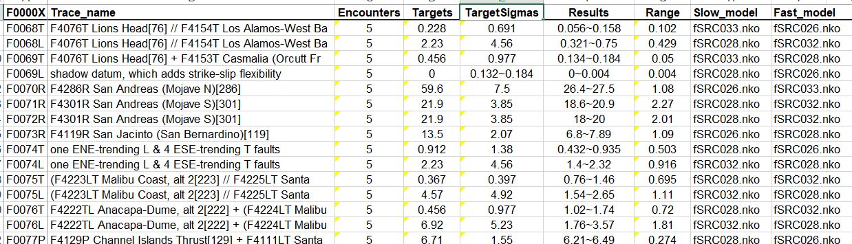
Notice that the rates quoted in this table are not slip-rates, but offset-rates
(of type indicated by the X in the F0000X fault-trace-index; i.e., L, R,
N, D, P, T, S).
Therefore, faults with oblique slip-rates will appear twice, in two adjacent
rows of the table.
(Experience shows that this format is preferable to showing ranges of slip
rates and rake angles; the latter may look “crazy” when both offset-rate
components are quite slow.)
Finally, let us consider the qualifier, “average
slip-rate of each fault.”
If you used a fine-grained F-E grid (.feg file), then probably
most of the faults that you modeled cross several finite-elements.
Within NeoKinema, a different offset-rate is computed in each element;
these are then averaged along the fault trace.
If you want to see all the local variations in heave-rates, there are two ways
to access that detail:
Ø The output file h*.nko
lists heave-rates by element.
(Admittedly, it is not in a very human-friendly format.)
Ø Mapping program NeoKineMap
has an option to display this fine detail, if you wish.
When you select Overlay # 6 :: “fault
heave rates (according to NeoKinema)”
you will next be asked to choose your preferred format:
---------------------------------------------------
Choose Presentation Method for Model Heave-Rates:
1: elegant plot, using trace-average rates
2: detailed plot, of individual segment rates
---------------------------------------------------
Which presentation method? [1]:
The following figure from Bird [2009] shows a comparison of these
formats:
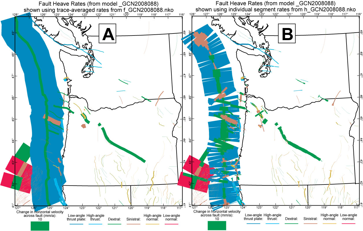
Occasionally this extra information may be interesting. For example, Figure
B above shows how the strike-slip component
on the long Cascadia subduction zone may change from right-lateral (green) to
left-lateral (brown) as you go North into Canada.
However, many of the other variations in B do not have clearly identifiable
physical causes, and perhaps should just be
explained as due to “discretization error” (that occurs when we substitute a
set of finite-elements for a continuum).
For most purposes, I prefer to report the trace-averaged heave-rate (or slip-rate)
which is probably more stable and reliable.
![]()
![]()
![]()
![]()
![]()