Step 39: Test your long-term SHIFT seismicity model retrospectively?

{If you did NOT create a SHIFT seismicity model in the previous Step, then this Step does not apply.
In that case, go directly on to the last Step.}

Many other forecasts of seismicity are created by smoothing and/or modeling seismic catalogs of recent earthquakes,
so as to extrapolate that seismicity into the future.  Testing such forecasts against the catalog(s) used to create them
would be circular and invalid.  Instead, one either has to reserve the last years of the catalog for testing,
or else wait many years until enough new catalog years become available for testing.

In contrast, SHIFT forecasts do not use seismic catalogs.  They are based on independent datasets such as
GPS velocities, fault traces, geologic offset rates, stress directions, and plate tectonics.  Therefore, any new
SHIFT forecast can immediately be tested retrospectively using any existing seismic catalog
(as long as that catalog is reasonably complete, accurate, unbiased, …).

Preparing the test-catalog dataset:

Whatever the source of your seismic catalog, it must be prepared, in two ways, for use in this Step:

(1) Conversion to my .eqc (EarthQuake Catalog) file format, which is documented here.

(2) Exclude unwanted earthquakes, which are either:
-outside the (longitude, latitude) rectangle of the seismicity forecast; and/or
-deeper than 70 km below sea level; and/or
-smaller than the threshold magnitude of the catalog (and the seismicity forecast).

Once you have performed the conversion step (1), you can use my utility program Seismicity to accomplish
the exclusion step (2), because Seismicity can read any .eqc file, apply exclusion rules, and then produce
a smaller output .eqc file.  (Seismicity will also offer to produce a simple .ai map-plot, but this is optional.)

Or, if you want to test against the Global Centroid Moment Tensor (GCMT) catalog, you can use GCMT
data file GCMT_1976_through_2017.ndk with Seismicity, and no conversion step will be needed.

Subjective graphical test:

Everyone wants to see actual earthquakes plotted on the same map as the forecast, to get an immediate
visual impression of whether the forecast has merit.  Although such comparisons are subjective and not
conclusive, they are an important way to discover whether or not your forecast has systematic defects.

Simply repeat the plot of the forecast (LTS_*.grd) file with NeoKineMap (as described in the previous Step),
and then add Overlay #14 :: earthquake epicenters from EarthQuake Catalog .eqc file.
If your test .eqc file contains focal-mechanism information (in the form of plunges & azimuths of P, B, & T axes),
you will have an option to plot the focal mechanisms using traditional lower-focal-hemisphere projections:

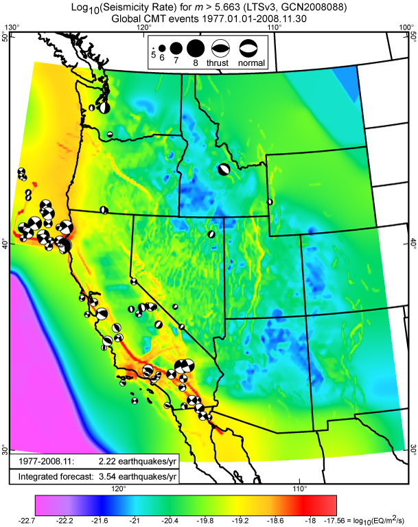
This is Figure 21 from Bird [2009].
Here you can see that I also made the plot a little bit more informative by computing the annual earthquake
rate from my .eqc file, and plotting that rate in a black-bordered white rectangle (inside Adobe Illustrator).
(Or, sometimes I like to convert both rates to “earthquakes per century” to emphasize that this is a long-term forecast.)

Formal testing with CSEP software:

The most widely-recognized formal tests of seismicity forecasts are those performed by the
Collaboratory for the Study of Earthquake Predictability (CSEP).
This is a non-profit, multi-institution, international testing group.
If your model fits into a predefined Testing Region (geographic) and model “class”, and is
presented with proper documentation and in proper file format, then independent seismologists
will test it (at no charge to you) in their computer center(s).
They will apply several absolute tests (e.g., N-test, L-test, M-test, S-test) of whether your forecast
can be distinguished from reality with high confidence (which would be a bad thing!).
If there are other competing forecasts in the same Test Region and model class, they will also
run some comparative tests (e.g., R-test) to see which forecast is better.
{The CSEP web site offers references to scientific papers which define all these tests.}

In the past, CSEP has primarily offered prospective testing (meaning that your forecast will only
be compared to earthquakes occurring after it has been installed at a CSEP testing center).
This involves a long wait for results!  However, there has been recent discussion about offering
more retrospective testing services through CSEP, so this could change in the future.

If you are in a hurry, or if you want to have more control of the testing process,
or if you want to quickly test many variants of your model, note that CSEP also offers
free downloads of their testing software.  The last time I checked, you needed to have a 64-bit Unix
workstation with lots of memory and disk space in order to install this download.

Informal testing with PseudoCSEP software:

I can also offer a simpler, “quick-and-dirty” version of many CSEP tests with my own program PseudoCSEP.
I wrote this for a number of reasons:

Ø Desire to understand the testing procedures more thoroughly.

Ø Desire for a product that runs under the Windows (32-bit or 64-bit) operating system, with parallel processing.

Ø Desire for the convenience of reading forecasts as .grd files, and reading test catalogs as .eqc files.

Ø Desire to exclude some features that I do not need (e.g., multiple magnitude-bins; multiple depth-bins).

Ø Desire to exclude some features that I believe to be misguided (e.g., declustering; addition of random noise to test-catalogs).

SO, I offer this software on a “buyer-beware; use at your own risk!” basis.
Whether reviewers of scientific manuscripts (or proposals) will find it convincing, I cannot say.

Some cautions, about systematic problems in CSEP testing of long-term forecasts:

The theoretical foundation under the “CSEP tests” (whether official or unofficial) is that they are
“likelihood-based tests” which return formal confidence values.
(For example, the N-test might tell you that there is, “95% confidence that your forecast has too many earthquakes.”).
All the formulas for “likelihood” (that these tests employ) assume that all the test earthquakes are independent.
That means that the test catalog should really be “declustered” (to remove all aftershocks), and the forecast
should also be “declustered”.  Unfortunately, there is no agreement on the proper algorithm for declustering,
and also it is very hard to understand how to “decluster” a long-term forecast of gridded seismicity rates,
where no specific events are forecast.

Thus, the apparent “precision” of the CSEP tests may be an illusion, especially for long-term gridded forecasts.
Worse, there can be a bias in the results if the declustering step is simply skipped:
Then, the CSEP algorithms will always tend to return a higher confidence than is really warranted.
(This is because they assume that all test earthquakes occurring in a forecast low-seismicity region are
equally bad news.  However, if only the first of these was independent, and the other were aftershocks,
the damage to the success of that forecast should have been less.)
Without declustering, CSEP tests will reject some forecasts unfairly.

Another issue is that most of the CSEP tests are designed to tell whether the forecast can be distinguished from reality.
The answer is usually No when the test catalog is short, converting eventually to Yes as the test gets longer.
But this is not very useful information for the modeler who is trying to incrementally improve their forecast.
Only a few of the CSEP tests answer the more important question, “Which of these alternative forecasts is better?”

For this reason, my group has tended to put more weight on an alternative comparative test that does not involve likelihood:

Comparative forecast testing with the Kagan information score:

The Kagan [2009, Geophys. J. Int.; equation (7)] information score I₁ is a simple metric for the relative success of
the map patterns of any seismicity forecasts with the same spatial extent and the same earthquake-selection rules.
Because it does not require declustering of either the forecast or the test catalog, it is particularly appropriate for forecasts of total seismicity.

This score can be described in words as the mean (over all test earthquakes) of the epicentroidal cell’s information gain
(expressed as the number of binary bits, including fractional bits) in the forecast under test,
relative to a reference model that has equal seismicity spread uniformly across the forecast domain.
This normalization by a reference model makes the ratio of earthquake rate densities dimensionless,
and also makes this I₁ metric completely insensitive to the total rate of earthquakes forecast (which should be tested separately).

This I₁ metric has several advantages:

Ø Forecasts of total seismicity are handled easily (more easily than mainshock forecasts).

Ø No changes are made to the test catalog (no declustering; no random perturbations).

Ø No simulations of virtual catalogs (based on the forecast) are needed.

Ø Computation involves no parameter choices and is very fast.

Ø Finite-test effects are benign; Kagan [2009] showed that the distribution of I₁
(for one fixed static forecast, across different test time-windows)
approaches a Gaussian distribution as the number of test earthquakes increases.
This would be expected from the central limit theorem, as I₁ is defined
as an average over many quasi-independent random variables.

Ø Scores (and score differences) are separable by test earthquake,
for better insight about forecast strengths and weaknesses.

To try this method, download and run my program Kagan_2009_GJI_I_scores.
For your convenience, it reads one forecast in .grd format, and one test catalog in .eqc format.
(It can also read an additional .grd file and use it for “windowing” the test, in case you want to compare
actual vs. forecast earthquake rates in some geographic region that is not rectangular.)
Its run-time is very short, and it produces a log-file for a lasting record of results.
To compare the performance of alternative forecasts, you simply run Kagan_2009_GJI_I_scores
once for each forecast, providing the same .eqc test-catalog each time.

An example of (ongoing) comparative testing of several global forecasts was given by Bird [2018].