![]()
![]()
![]()
![]()
![]()
Step 38: Run Long_Term_Seismicity to get a SHIFT seismicity model?
Bird
& Liu [2007] stated a pair
of hypotheses for a group of seismicity-estimation methods known by the
acronym SHIFT (Seismic Hazard Inferred From Tectonics):
(1)
The long-term seismic moment rate of any tectonic fault, or any large
volume of permanently deforming lithosphere,
is approximately that computed using the coupled seismogenic thickness of the
most comparable type of plate boundary, and
(2) The
long-term seismicity of any tectonic fault, or any large volume of permanently
deforming lithosphere,
is approximately that computed from its moment rate using the
frequency-magnitude distribution of the most comparable type of plate boundary.
That is, even faults of modest length and slip-rate (which would not ever be
considered “plate boundaries”) can be
approximated as plate boundaries for purposes of estimating their seismicity
(per unit length, and per unit slip-rate),
provided that the seismicity of all the “classic” plate-boundary types has been
calibrated using only accepted, unambiguous plate boundaries.
Previously, Bird [2003] had presented the PB2002 model
of the locations of plate boundaries, recognizing 52 plates and 13 orogens.
This enabled Bird &
Kagan [2004] to determine the
seismicity coefficients of the 7 different classes of plate boundary, while
avoiding the complex, poorly-known orogens of Bird [2003], and using the
Global Centroid Moment Tensor (GCMT)
seismic catalog which has uniform global coverage and an accurate seismic
moment for each event above its threshold (m ≥ 5.7).
One important qualification to the SHIFT hypotheses was later discovered by Bird
et al. [2009]:
Only certain classes of plate boundary (continental and oceanic transform
faults, continental rifts, & oceanic convergent boundaries)
have seismicity in strict proportion to relative plate velocity; the other
classes (subduction zones, continental convergence zones,
and mid-ocean spreading ridges) have nonlinear relations between seismicity and
relative plate velocity.
This clarified that the analog plate boundaries most appropriate for relatively
slow-moving faults in orogens
are the slowest subduction zones, continental convergent boundaries, and ridges
(not the global averages of those 3 classes).
After this calibration was finished, it became relatively straightforward to
convert fault slip-rates and permanent strain-rates
from any kinematic (or dynamic) model of neotectonics into a map of
long-term-average shallow seismicity.
To date, the SHIFT method has been applied in two models of the neotectonics of
California [Bird
& Liu, 2007; Bird, 2009],
in two models of the southern-Europe/Mediterranean region [Howe & Bird, 2010; Carafa
et al., 2017],
and in two global models [Bird et al., 2010; Bird &
Kreemer, 2015]. The latter
global model was also a
“parent model” component of the GEAR1 global seismicity model of Bird et al. [2015].
The utility program that converts any preferred NeoKinema model to
seismicity is Long_Term_Seismicity.
It produces a rectangular grid, in (longitude, latitude) coordinates, of
earthquake-rate densities (per unit area),
expressed as shallow centroids per meter-squared per second. These values
are arranged into a .grd file,
whose format is documented here.
In a slight extension of the .grd format, title lines (recording the
chosen threshold magnitude)
are included in the right-hand portions of the first two records.
Also, two kinds of summary information are also included at the bottom of the
file:
Ø The spatial integral, or total shallow (z £ 70 km) seismicity rate, above threshold magnitude, of the model.
Ø The fraction of seismicity coming from
slip on modeled faults, versus the fraction coming from
permanent deformation of unfaulted(?) “continuum” or “microplate” elements.
Now, most orogens modelled with NeoKinema are not rectangular. This presented a dilemma:
a) Should seismicity models be limited to rectangular regions lying entirely within each NeoKinema model? OR,
b) Should other kinematic (or dynamic) models be used to estimate seismicity in the margins of the rectangle?
Program Long_Term_Seismicity takes the second option, (b). In every run, it reads extra input files so that it is prepared to use:
Ø The global PB2002 model of 52 rigid
plates by Bird [2003]
(for plate-boundary locations and relative plate velocities); and/or
Ø The preferred Shells-based global
dynamic model Earth5-049 of Bird et
al. [2008]
(for long-term-average permanent-strain-rates of plate interiors).
If it actually finds that the rectangular region of the requested seismicity
model is entirely within the NeoKinema model,
then these alternative estimates of surface kinematics will be overwritten by
kinematics from NeoKinema.
Long_Term_Seismicity also requires two global datasets that are used
to decide which grid points have “oceanic” lithosphere,
and which points are “continental.” The file ETOPO5.grd contains
a digital elevation model (DEM) that was created by NOAA.
The file age_1p5.grd
contains gridded ages of seafloor (based on linear magnetic anomalies) from Mueller
et al. [1997, JGR].
The rule is that a grid point is “oceanic” if it has an age < 180 Ma, OR if
it is under more than 2 km of water;
all other points are “continental” (even if under shallow seas).
Long_Term_Seismicity is actually very easy to use. The user only has to specify (from the keyboard):
§ A choice of alternative (global or
regional) seismicity coefficients to be applied;
(The references corresponding to these options are:
0: global or default settings: Bird &
Kagan [2004]
1: western United States settings: Bird &
Kagan [2004]
2: Italia settings: Carafa
et al. [2017]
3: SyntheticExample: Bird
& Carafa [2016]
{all-continental; no global datasets})
§ A choice of output file formats (I suggest .grd);
§ The threshold magnitude (usually 5.0 or
higher, on the moment-magnitude scale;
it should equal the completeness-threshold magnitude of the seismic catalog
that you intend to use for testing in the next Step);
§ The (longitude, latitude) limits of the desired map-rectangle;
§ The desired grid-spacing in degrees (e.g., 0.1° £ 11 km, or: 0.04° £ 4.4 km); and
§ The desired name for the output (e.g., LTS_*.grd) grid file.
So, in practice, the main work of running Long_Term_Seismicity is
just the job of collecting the necessary input files
into one folder, which will be the active folder when this utility is started:
|
F-E grid used by Bird et al. [2008] to compute Shells model Earth5-049 |
|
|
Node velocities obtained by Bird et al. [2008] from Shells model Earth5-049 |
|
|
Step-wise table representation of plate-boundary locations, classes, and relative velocities, from PB2002 model of Bird [2003] |
|
|
f*.dig |
Input to your preferred NeoKinema model: digitized fault traces (& dips?) |
|
*.feg |
Input to your preferred NeoKinema model: F-E grid |
|
e*.nko |
Output from your preferred NeoKinema modal: strain-rates in elements |
|
h*.nko |
Output from your preferred NeoKinema model: fault heave-rates, by element |
|
Global topography dataset at 5’ resolution |
|
|
Gridded ages of global seafloor, by Mueller et al. [1997] |
As shown by the hyperlinks in the table above, all the left-justified files
are available from this web site.
You only need to provide the 4 right-justified files, from your preferred NeoKinema
model (“*”).
Once Long_Term_Seismicity
has finished, it is very easy to plot the seismicity .grd with NeoKineMap;
just request Mosaic #10 ::
logarithm of seismicity rate, from a Long_Term_Seismicity .grd file.
THEN:
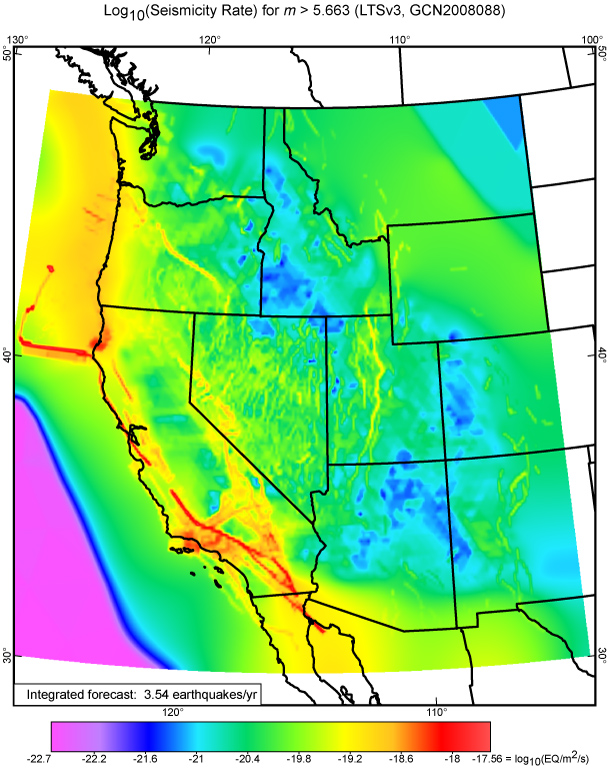
The map above is Figure 20 from Bird [2009]. Obviously, the map also
includes an
Overlay of type #1: North_America_states.dig.
![]()
![]()
![]()
![]()
![]()